[math] \require{textmacros} \def \bbeta {\bf \beta} \def\fat#1{\mbox{\boldmath$#1$}} \def\reminder#1{\marginpar{\rule[0pt]{1mm}{11pt}}\textbf{#1}} \def\SSigma{\bf \Sigma} \def\ttheta{\bf \theta} \def\aalpha{\bf \alpha} \def\ddelta{\bf \delta} \def\eeta{\bf \eta} \def\llambda{\bf \lambda} \def\ggamma{\bf \gamma} \def\nnu{\bf \nu} \def\vvarepsilon{\bf \varepsilon} \def\mmu{\bf \mu} \def\nnu{\bf \nu} \def\ttau{\bf \tau} \def\SSigma{\bf \Sigma} \def\TTheta{\bf \Theta} \def\XXi{\bf \Xi} \def\PPi{\bf \Pi} \def\GGamma{\bf \Gamma} \def\DDelta{\bf \Delta} \def\ssigma{\bf \sigma} \def\UUpsilon{\bf \Upsilon} \def\PPsi{\bf \Psi} \def\PPhi{\bf \Phi} \def\LLambda{\bf \Lambda} \def\OOmega{\bf \Omega} [/math]
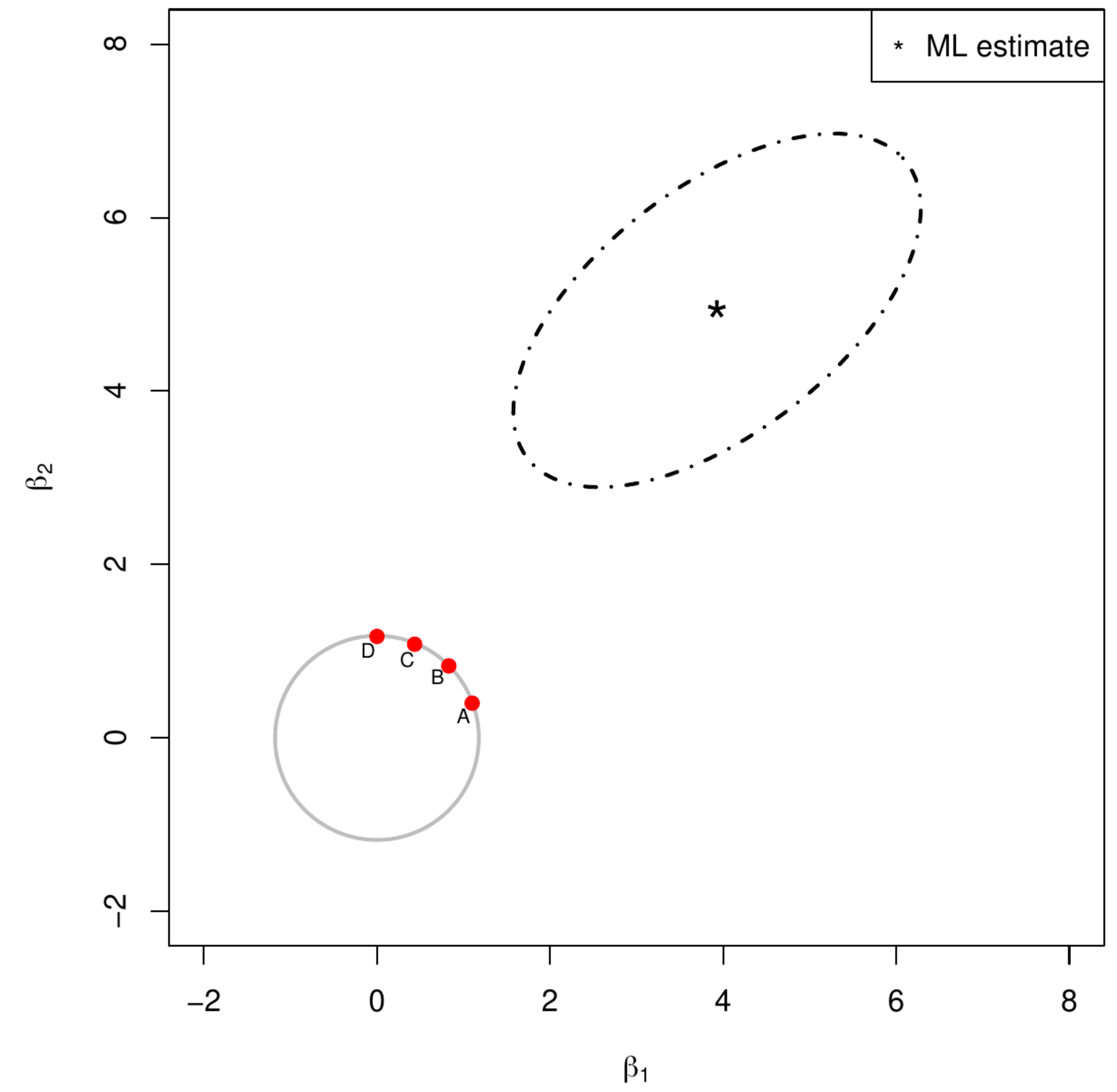
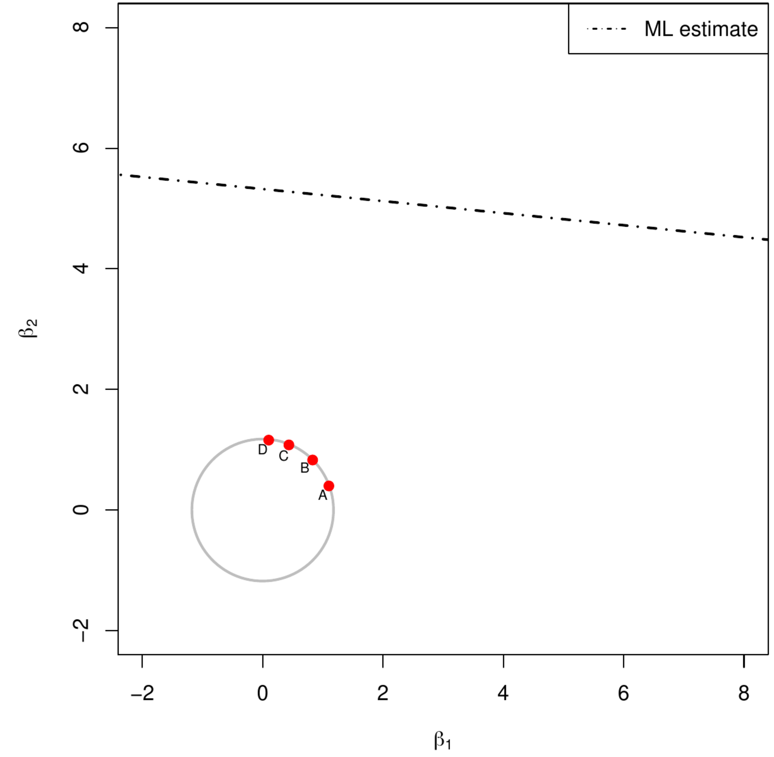
The ridge regression estimator can be viewed as the solution of a constraint estimation problem. Consider the two panels of Figure. Both show the ridge parameter constraint represented by the grey circle around the origin. The left panel also contains an ellopsoid representing a level set of the sum-of-squares centered around the maximum likelihood regression estimate, while the right panel contains a line formed by the solutions of the normal equations. Both panels have four red dots on the boundary of the ridge parameter constraint. Identify for both cases, which of these four dots is (closest to) the ridge regression estimate?
[math] \require{textmacros} \def \bbeta {\bf \beta} \def\fat#1{\mbox{\boldmath$#1$}} \def\reminder#1{\marginpar{\rule[0pt]{1mm}{11pt}}\textbf{#1}} \def\SSigma{\bf \Sigma} \def\ttheta{\bf \theta} \def\aalpha{\bf \alpha} \def\ddelta{\bf \delta} \def\eeta{\bf \eta} \def\llambda{\bf \lambda} \def\ggamma{\bf \gamma} \def\nnu{\bf \nu} \def\vvarepsilon{\bf \varepsilon} \def\mmu{\bf \mu} \def\nnu{\bf \nu} \def\ttau{\bf \tau} \def\SSigma{\bf \Sigma} \def\TTheta{\bf \Theta} \def\XXi{\bf \Xi} \def\PPi{\bf \Pi} \def\GGamma{\bf \Gamma} \def\DDelta{\bf \Delta} \def\ssigma{\bf \sigma} \def\UUpsilon{\bf \Upsilon} \def\PPsi{\bf \Psi} \def\PPhi{\bf \Phi} \def\LLambda{\bf \Lambda} \def\OOmega{\bf \Omega} [/math]
Consider the standard linear regression model [math]Y_i = \mathbf{X}_{i,\ast} \bbeta + \varepsilon_i[/math] for [math]i=1, \ldots, n[/math] and with the [math]\varepsilon_i[/math] i.i.d. normally distributed with zero mean and a common variance. The rows of the design matrix [math]\mathbf{X}[/math] have two elements, and neither column represents the intercept, but [math]\mathbf{X}_{\ast, 1} = \mathbf{X}_{\ast, 2}[/math].
- Suppose an estimator of the regression parameter [math]\bbeta[/math] of this model is obtained through the minimization of the sum-of-squares augmented with a ridge penalty, [math]\| \mathbf{Y} - \mathbf{X} \bbeta \|_2^2 + \lambda \| \bbeta \|_2^2[/math], in which [math]\lambda \gt 0[/math] is the penalty parameter. The minimizer is called the ridge estimator and is denoted by [math]\hat{\bbeta}(\lambda)[/math]. Show that [math][\hat{\bbeta}(\lambda)]_1 = [\hat{\bbeta}(\lambda)]_2[/math] for all [math]\lambda \gt 0[/math].
- The covariates are now related as [math]\mathbf{X}_{\ast, 1} = - 2 \mathbf{X}_{\ast, 2}[/math]. Data on the response and the covariates are:
[[math]] \begin{eqnarray*} \{(y_i, x_{i,1}, x_{i,2})\}_{i=1}^6 & = & \{ (1.5, 1.0, -0.5), (1.9, -2.0, 1.0), (-1.6, 1.0, -0.5), \\ & & \, \, \, (0.8, 4.0, -2.0), (0.9, 2.0, -1.0), (\textcolor{white}{-} 0.5, 4.0, -2.0) \}. \end{eqnarray*} [[/math]]Evaluate the ridge regression estimator for these data with [math]\lambda = 1[/math].
- The data are as in part b). Show [math]\hat{\bbeta}(\lambda+\delta) = (52.5 + \lambda) (52.5 + \lambda + \delta)^{-1} \hat{\bbeta}(\lambda)[/math] for a fixed [math]\lambda[/math] and any [math]\delta \gt 0[/math]. That is, given the ridge regression estimator evaluated for a particular value of the penalty parameter [math]\lambda[/math], the remaining regularization path [math]\{ \hat{\bbeta}(\lambda + \delta) \}_{\delta \geq 0}[/math] is known analytically. Hint: Use the singular value decomposition of the design matrix [math]\mathbf{X}[/math] and the fact that its largest singular value equals [math]\sqrt{52.5}[/math].
- The data are as in part b). Consider the model [math]Y_i = X_{i,1} \gamma + \varepsilon_i[/math]. The parameter [math]\gamma[/math] is estimated through minimization of [math]\sum_{i=1}^6 (Y_i - X_{i,1} \gamma)^2 + \lambda_{\gamma} \gamma^2[/math]. The perfectly linear relation of the covariates suggests that the regularization paths of the linear predictors [math]X_{i,1} \hat{\gamma}(\lambda_{\gamma})[/math] and [math]\mathbf{X}_{i,\ast} \hat{\bbeta}(\lambda)[/math] overlap. Find the functional relationship [math]\lambda_{\gamma} = f(\lambda)[/math] such that the resulting linear predictor [math]X_{i,1} \hat{\gamma}(\lambda_{\gamma})[/math] indeed coincides with that obtained from the estimate evaluated in part b) of this exercise, i.e. [math]\mathbf{X} \hat{\bbeta}(\lambda)[/math].
[math] \require{textmacros} \def \bbeta {\bf \beta} \def\fat#1{\mbox{\boldmath$#1$}} \def\reminder#1{\marginpar{\rule[0pt]{1mm}{11pt}}\textbf{#1}} \def\SSigma{\bf \Sigma} \def\ttheta{\bf \theta} \def\aalpha{\bf \alpha} \def\ddelta{\bf \delta} \def\eeta{\bf \eta} \def\llambda{\bf \lambda} \def\ggamma{\bf \gamma} \def\nnu{\bf \nu} \def\vvarepsilon{\bf \varepsilon} \def\mmu{\bf \mu} \def\nnu{\bf \nu} \def\ttau{\bf \tau} \def\SSigma{\bf \Sigma} \def\TTheta{\bf \Theta} \def\XXi{\bf \Xi} \def\PPi{\bf \Pi} \def\GGamma{\bf \Gamma} \def\DDelta{\bf \Delta} \def\ssigma{\bf \sigma} \def\UUpsilon{\bf \Upsilon} \def\PPsi{\bf \Psi} \def\PPhi{\bf \Phi} \def\LLambda{\bf \Lambda} \def\OOmega{\bf \Omega} [/math]
Consider the standard linear regression model [math]Y_i = \mathbf{X}_{i,\ast} \bbeta + \varepsilon_i[/math] for [math]i=1, \ldots, n[/math] and with the [math]\varepsilon_i[/math] i.i.d. normally distributed with zero mean and a common variance. Moreover, [math]\mathbf{X}_{\ast,j} = \mathbf{X}_{\ast,j'}[/math] for all [math]j, j'=1, \ldots, p[/math] and [math]\sum_{i=1}^n X_{i,j}^2 = 1[/math]. Show that the ridge regression estimator, defined as [math]\bbeta(\lambda_2) = \arg \min_{\bbeta \in \mathbb{R}^p} \| \mathbf{Y} - \mathbf{X} \bbeta \|_2^2 + \lambda \| \bbeta \|_2^2[/math] for [math]\lambda \gt 0[/math], equals:
where [math]b = \mathbf{X}_{\ast,1}^{\top} \mathbf{Y}[/math]. Hint: you may want to use the Sherman-Morrison formula. Let [math]\mathbf{A}[/math] and [math]\mathbf{B}[/math] be symmetric matrices of the same dimension, with [math]\mathbf{A}[/math] invertible and [math]\mathbf{B}[/math] of rank one. Moreover, define [math]g = \mbox{tr}( \mathbf{A}^{-1} \mathbf{B})[/math]. Then: [math](\mathbf{A} + \mathbf{B})^{-1} = \mathbf{A}^{-1} - (1+g)^{-1} \mathbf{A}^{-1} \mathbf{B} \mathbf{A}^{-1}[/math].
[math] \require{textmacros} \def \bbeta {\bf \beta} \def\fat#1{\mbox{\boldmath$#1$}} \def\reminder#1{\marginpar{\rule[0pt]{1mm}{11pt}}\textbf{#1}} \def\SSigma{\bf \Sigma} \def\ttheta{\bf \theta} \def\aalpha{\bf \alpha} \def\ddelta{\bf \delta} \def\eeta{\bf \eta} \def\llambda{\bf \lambda} \def\ggamma{\bf \gamma} \def\nnu{\bf \nu} \def\vvarepsilon{\bf \varepsilon} \def\mmu{\bf \mu} \def\nnu{\bf \nu} \def\ttau{\bf \tau} \def\SSigma{\bf \Sigma} \def\TTheta{\bf \Theta} \def\XXi{\bf \Xi} \def\PPi{\bf \Pi} \def\GGamma{\bf \Gamma} \def\DDelta{\bf \Delta} \def\ssigma{\bf \sigma} \def\UUpsilon{\bf \Upsilon} \def\PPsi{\bf \Psi} \def\PPhi{\bf \Phi} \def\LLambda{\bf \Lambda} \def\OOmega{\bf \Omega} [/math]
Consider the linear regression model [math]\mathbf{Y} = \mathbf{X} \bbeta + \vvarepsilon[/math], without intercept and [math]\vvarepsilon \sim \mathcal{N} ( \mathbf{0}_n, \sigma^2 \mathbf{I}_{nn})[/math], to explain the variation in the response [math]\mathbf{Y}[/math] by a linear combination of the columns of the design matrix [math]\mathbf{X}[/math]. The linear regression model is fitted by means of ridge estimation. The estimator is evaluated directly from its regular expression and a computationally efficient one:
respectively. In the remainder study the computational gain of the latter. Hereto carry out the following instructions:
- Load the R-package microbenchmark [1].
- Generate data. In this fix the sample size at [math]n=10[/math], and let the dimension range from [math]p=10, 20, 30, \ldots, 100[/math]. Sample the elements of the response and the ten design matrices from the standard normal distribution.
- Verify the superior computation time of the latter by means of the microbenchmark-function with default settings. Throughout use the first design matrix and [math]\lambda=1[/math]. Write the output of the microbenchmark-function to an R-object. It will be a data.frame with two slots expr and time that contain the function calls and the corresponding computation times, respectively. Each call has by default been evaluated a hundred times in random order. Summary statistics of these individual computation times are given when printing the object on the screen.
- Use the crossprod- and tcrossprod-functions to improve the computation times of the evaluation of both [math]\hat{\bbeta}_{\mbox{{\tiny reg}}} (\lambda)[/math] and [math]\hat{\bbeta}_{\mbox{{\tiny eff}}} (\lambda)[/math] as much as possible.
- Use the microbenchmark-function to evaluate the (average) computation time both [math]\hat{\bbeta}_{\mbox{{\tiny reg}}} (\lambda)[/math] and [math]\hat{\bbeta}_{\mbox{{\tiny eff}}} (\lambda)[/math] on all ten data sets, i.e. defined by the ten design matrices with different dimensions.
- Plot, for both [math]\hat{\bbeta}_{\mbox{{\tiny reg}}} (\lambda)[/math] and [math]\hat{\bbeta}_{\mbox{{\tiny eff}}} (\lambda)[/math], the (average) computation time (on the [math]y[/math]-axis) against the dimension of the ten data sets. Conclude on the computation gain from the plot.

