guide:E8d7c0f552: Difference between revisions
No edit summary |
mNo edit summary |
||
| (One intermediate revision by one other user not shown) | |||
| Line 1: | Line 1: | ||
<div class="d-none"><math> | |||
\newcommand{\ex}[1]{\item } | |||
\newcommand{\sx}{\item} | |||
\newcommand{\x}{\sx} | |||
\newcommand{\sxlab}[1]{} | |||
\newcommand{\xlab}{\sxlab} | |||
\newcommand{\prov}[1] {\quad #1} | |||
\newcommand{\provx}[1] {\quad \mbox{#1}} | |||
\newcommand{\intext}[1]{\quad \mbox{#1} \quad} | |||
\newcommand{\R}{\mathrm{\bf R}} | |||
\newcommand{\Q}{\mathrm{\bf Q}} | |||
\newcommand{\Z}{\mathrm{\bf Z}} | |||
\newcommand{\C}{\mathrm{\bf C}} | |||
\newcommand{\dt}{\textbf} | |||
\newcommand{\goesto}{\rightarrow} | |||
\newcommand{\ddxof}[1]{\frac{d #1}{d x}} | |||
\newcommand{\ddx}{\frac{d}{dx}} | |||
\newcommand{\ddt}{\frac{d}{dt}} | |||
\newcommand{\dydx}{\ddxof y} | |||
\newcommand{\nxder}[3]{\frac{d^{#1}{#2}}{d{#3}^{#1}}} | |||
\newcommand{\deriv}[2]{\frac{d^{#1}{#2}}{dx^{#1}}} | |||
\newcommand{\dist}{\mathrm{distance}} | |||
\newcommand{\arccot}{\mathrm{arccot\:}} | |||
\newcommand{\arccsc}{\mathrm{arccsc\:}} | |||
\newcommand{\arcsec}{\mathrm{arcsec\:}} | |||
\newcommand{\arctanh}{\mathrm{arctanh\:}} | |||
\newcommand{\arcsinh}{\mathrm{arcsinh\:}} | |||
\newcommand{\arccosh}{\mathrm{arccosh\:}} | |||
\newcommand{\sech}{\mathrm{sech\:}} | |||
\newcommand{\csch}{\mathrm{csch\:}} | |||
\newcommand{\conj}[1]{\overline{#1}} | |||
\newcommand{\mathds}{\mathbb} | |||
</math></div> | |||
<span id ="sec_1.2"/> | |||
The set whose members consist of just the two elements <math>a</math> and <math>b</math> | |||
is denoted <math>\{ a, b \}</math>. | |||
The notation is not perfect because it suggests that the members <math>a</math> and <math>b</math> have been ordered: | |||
<math>a</math> is written first and <math>b</math> second. | |||
Actually no ordering is present because <math>\{ a, b \} = \{ b, a \}</math>. | |||
Note also that if <math>a = b</math>, | |||
then <math>\{ a, b \} = \{ b, a \} = \{ a \}</math>. | |||
It can happen, however, that the ingredient of order is essential. | |||
We therefore introduce the notion of | |||
an '''ordered pair''' <math>(a, b)</math> | |||
whose first member is <math>a</math> and whose second member is <math>b</math>. | |||
The characteristic property of ordered pairs is | |||
<math display="block"> | |||
(a, b) = (c, d) \provx{if and only if $a = c$ and $b=d$.} | |||
</math> | |||
In particular <math>(a, b) = (b, a)</math> ''if and only if'' <math>a = b</math>. | |||
In Section \secref{1.1} | |||
we saw that the set <math>\R</math> of all real numbers | |||
can be thought of as a straight line. | |||
We shall now show that every ordered pair <math>(a, b)</math> | |||
of real numbers <math>a</math> and <math>b</math> | |||
can be identified with a point in a plane. | |||
This brings up a notational problem: | |||
Is <math>(5, 7)</math> the ordered pair of real numbers | |||
or is it the open interval consisting of all <math>x</math> | |||
such that <math>5 < x < 7</math>? | |||
The answer is that it is impossible to tell | |||
out of context---just as it is impossible to tell whether the word | |||
“well” is the noun or the adverb. | |||
Consider two distinct real number lines drawn in a plane | |||
so that they intersect at the number <math>0</math> on each line. | |||
One of the lines is traditionally drawn horizontal | |||
and called the '''<math>x</math>-axis''', | |||
and the other is made perpendicular to it | |||
and called the '''<math>y</math>-axis'''. | |||
The orientation is chosen so that the number <math>1</math> on the <math>x</math>-axis | |||
lies to the right of <math>0</math>, | |||
and the number <math>1</math> on the <math>y</math>-axis is above <math>0</math>. | |||
It is also customary to use the same scale of distances on both axes. | |||
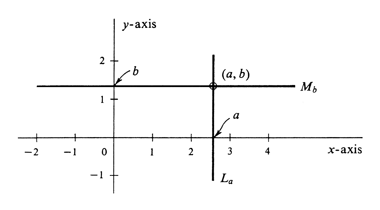
For every ordered pair <math>(a, b)</math> of real numbers, | |||
let <math>L_a</math> be the line parallel to the <math>y</math>-axis | |||
that cuts the <math>x</math>-axis at <math>a</math>, | |||
and let <math>M_b</math> be the line parallel to the <math>x</math>-axis | |||
that cuts the <math>y</math>-axis at <math>b</math>. | |||
We assign the point of intersection of <math>L_a</math> and <math>M_b</math> | |||
to the ordered pair <math>(a, b)</math> (see [[#fig 1.6|Figure]]). | |||
The numbers <math>a</math> and <math>b</math> are called the '''coordinates''' of the point. | |||
<math>a</math> is the '''<math>x</math>-coordinate''' | |||
(or '''abscissa''') | |||
and <math>b</math> is the '''<math>y</math>-coordinate''' | |||
(or '''ordinate'''). | |||
<div id="fig 1.6" class="d-flex justify-content-center"> | |||
[[File:guide_c5467_scanfig1_6.png | 400px | thumb | ]] | |||
</div> | |||
If the pairs <math>(a, b)</math> and <math>(c, d)</math> are not equal, | |||
then the points in the plane assigned to them will be different. | |||
In addition, every point in the plane has a number pair assigned to it: | |||
Starting with a point, draw the two lines through it | |||
which are parallel to the <math>x</math>-axis and the <math>y</math>-axis. | |||
One line cuts the <math>x</math>-axis at a number <math>a</math>, | |||
and the other cuts the <math>y</math>-axis at <math>b</math>. | |||
The ordered pair <math>(a, b)</math> has the original point assigned to it. | |||
It follows that our assignment | |||
<math display="block"> | |||
\mbox{pair} \goesto \mbox{point} | |||
</math> | |||
is a one-to-one correspondence | |||
between the set of all ordered pairs of real numbers, | |||
which we denote by <math>\R^2</math>, | |||
and the set of all points of the plane. | |||
It is convenient simply to identify <math>\R^2</math> with the plane | |||
together with the two axes. | |||
<span id="exam 1.2.1"/> | |||
'''Example''' | |||
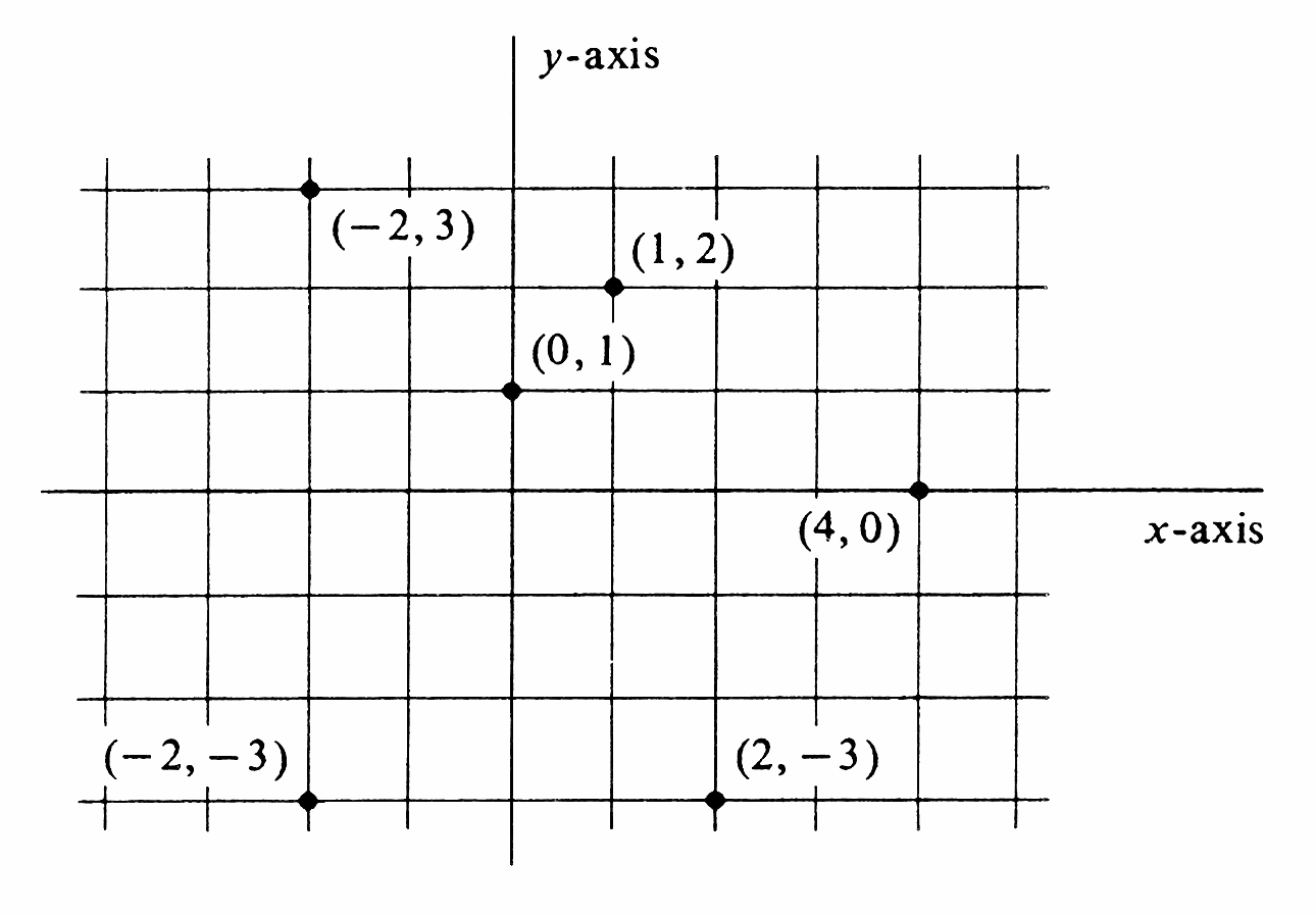
Plot the points | |||
<math>(1, 2), (-2, 3), (0, 1), (4, 0), (-2, -3)</math>, and <math>(2, -3)</math> | |||
on the <math>xy</math>-plane | |||
(see [[#fig 1.7|Figure]]). | |||
<div id="fig 1.7" class="d-flex justify-content-center"> | |||
[[File:guide_c5467_scanfig1_7.png | 400px | thumb | ]] | |||
</div> | |||
The usefulness of the idea of an ordered pair | |||
is by no means limited to pairs of real numbers. | |||
In plane geometry, for example, | |||
we may consider the set of all ordered pairs <math>(T, p)</math> | |||
in which <math>T</math> is a triangle and <math>p</math> is the point of intersection | |||
of its medians. | |||
In the three-dimensional extension of the <math>xy</math>-plane, | |||
the set <math>\R^3</math> of all ordered triples <math>(a, b, c)</math> of real numbers | |||
is identified with the set of all points in three-dimensional space. | |||
The definition of an ordered triple | |||
can be reduced to that of an ordered pair | |||
by defining <math>(a, b, c)</math> to be <math>((a, b), c)</math>. | |||
<div id="fig 1.8" class="d-flex justify-content-center"> | |||
[[File:guide_c5467_scanfig1_8.png | 400px | thumb | ]] | |||
</div> | |||
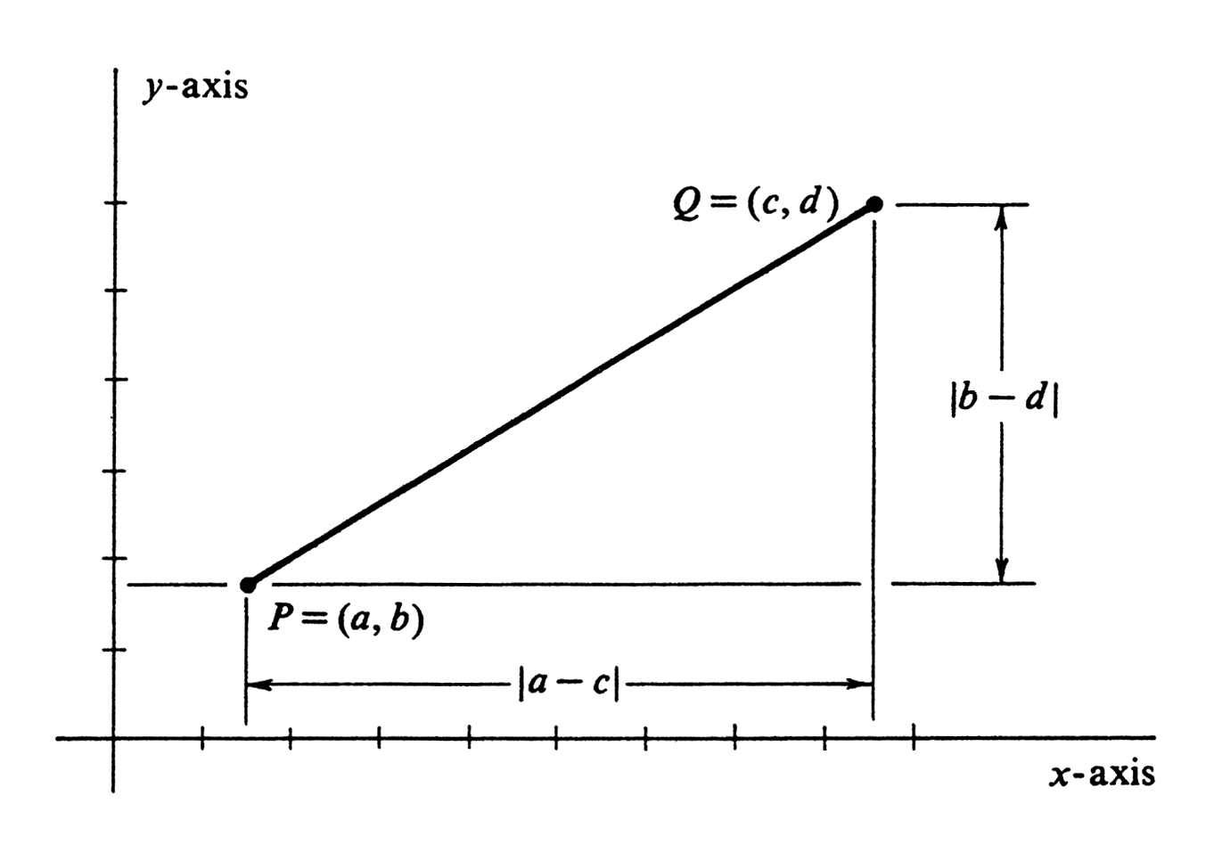
Let <math>P = (a, b)</math> and <math>Q = (c, d)</math> | |||
be arbitrary elements in the set | |||
<math>\R^2</math> of all ordered pairs of real numbers. | |||
We define the '''distance''' between <math>P</math> and <math>Q</math> by the formula | |||
<span id{{=}}"eq1.2.1"/> | |||
<math display="block"> | |||
\begin{equation} | |||
\label{eq1.2.1} | |||
\dist(P, Q) = \sqrt{(a - c)^2 + (b - d)^2}. | |||
\end{equation} | |||
</math> | |||
Three simple corollaries of this definition are: | |||
{{proofcard|Proposition|thm_1.2.1|<math>\dist(P, Q) \geq 0</math>; i.e., distance is never negative.|}} | |||
{{proofcard|Proposition|thm_1.2.2|<math>\dist(P, Q) = 0</math> | |||
if and only if <math>P = Q</math>.|}} | |||
{{proofcard|Proposition|thm_1.2.3|<math>\dist(P, Q) = \dist (Q, P)</math>.|}} | |||
Another consequence of (1) | |||
is that it is no longer simply a matter of tradition and convenience | |||
that we draw the <math>y</math>-axis perpendicular to the <math>x</math>-axis. | |||
It follows from consideration of the Pythagorean Theorem | |||
and its converse (see [[#fig 1.8|Figure]]) | |||
that the above definition of distance between elements of <math>\R^2</math> | |||
corresponds with our geometric notion of the distance between points | |||
in the Euclidean plane | |||
if and only if the two coordinate axes are perpendicular | |||
and the scales are the same on both. | |||
<div id="fig 1.9" class="d-flex justify-content-center"> | |||
[[File:guide_c5467_scanfig1_9.png | 400px | thumb | ]] | |||
</div> | |||
<span id="exam 1.2.2"/> | |||
'''Example''' | |||
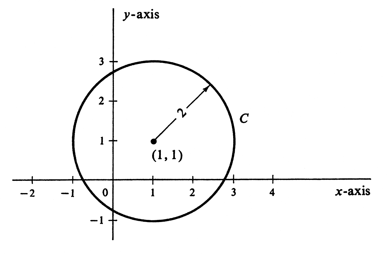
Let <math>C</math> be the subset of the <math>xy</math>-plane | |||
consisting of all points whose distance from (1,1) is equal to 2. | |||
Thus <math>C</math> is the circle shown in [[#fig 1.9|Figure]]. | |||
If <math>(x, y)</math> is an arbitrary point in the <math>xy</math>-plane, | |||
its distance from <math>(1,1)</math> | |||
is equal to | |||
<math>\sqrt{(x - 1)^2 + (y - 1)^2}</math>. | |||
Hence, <math>(x, y)</math> belongs to <math>C</math> | |||
if and only if | |||
<span id{{=}}"eq1.2.2"/> | |||
<math display="block"> | |||
\begin{equation} | |||
\sqrt{(x - 1)^2 + (y - 1)^2} = 2. | |||
\label{eq1.2.2} | |||
\end{equation} | |||
</math> | |||
Numbers <math>x</math> and <math>y</math> satisfy (2) | |||
if and only if they satisfy | |||
<span id{{=}}"eq1.2.3"/> | |||
<math display="block"> | |||
\begin{equation} | |||
(x - 1)^2 + (y - 1)^2 = 4. | |||
\label{eq1.2.3} | |||
\end{equation} | |||
</math> | |||
Thus <math>C</math> is the set of all ordered pairs <math>(x, y)</math> | |||
that satisfy (3)---or that satisfy (2). | |||
Either (2) or (3) is therefore called | |||
'''an equation of the circle''' <math>C</math>. | |||
The set of all points <math>(x, y)</math> in the plane | |||
that satisfy a given equation is called the | |||
'''graph''' of the equation. | |||
Hence, in the above example, | |||
the circle <math>C</math> is the graph of the equation | |||
<math>(x - 1)^2 + (y - 1)^2 = 4</math>. | |||
<span id="exam 1.2.3"/> | |||
'''Example''' | |||
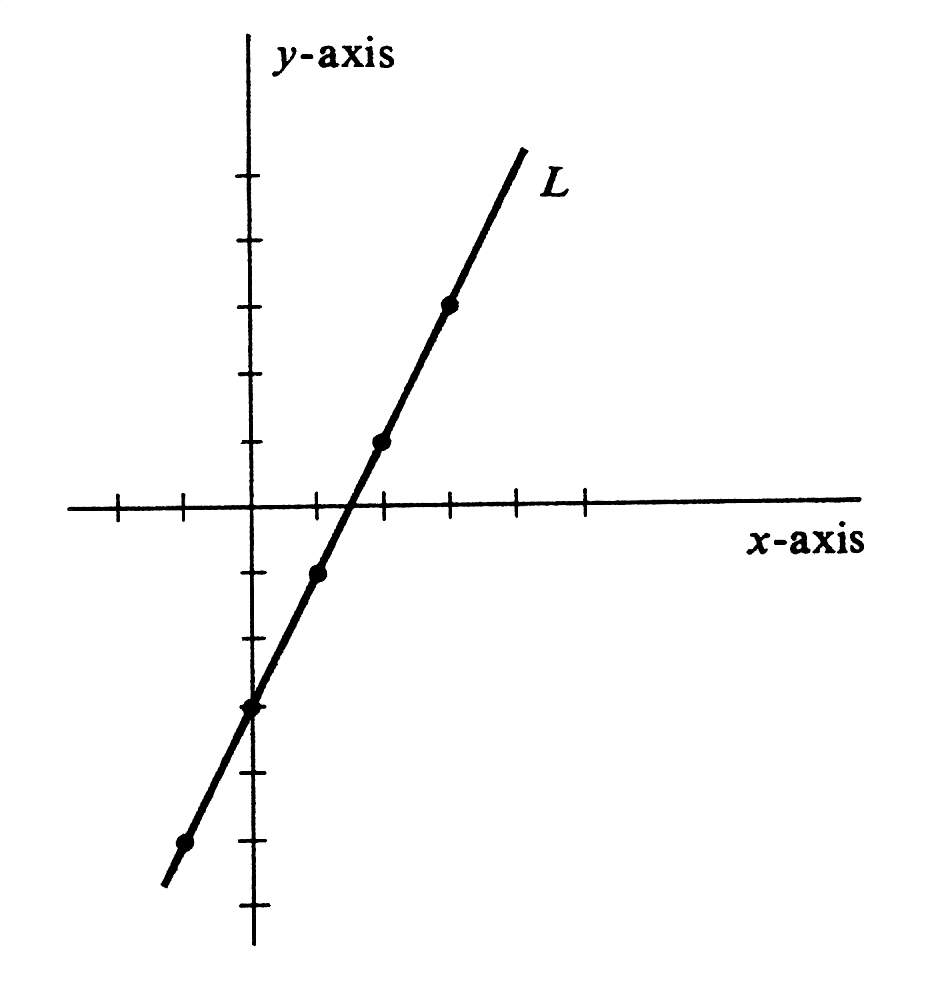
Let <math>L</math> be the set of all ordered pairs <math>(x, y)</math> | |||
such that <math>y = 2x - 3</math>. | |||
For each real number <math>x</math>, | |||
there is one and only one number <math>y</math> | |||
such that <math>(x, y)</math> belongs to <math>L: y = 2x - 3</math>. | |||
To see what <math>L</math> looks like, | |||
we plot five of its points (see [[#table 1.1 |Table]]). | |||
As shown in [[#fig 1.10|Figure]], | |||
all these points lie on a straight line. | |||
In Section \secref{1.5} | |||
we shall justify the natural conjecture | |||
that this straight line is the set <math>L</math>. | |||
<span id="table 1.1"/> | |||
{|class="table" | |||
|- | |||
|<math>x</math> || <math>y=2x - 3</math> | |||
|- | |||
|-1 || -5 | |||
|- | |||
|0 || -3 | |||
|- | |||
|1 || -1 | |||
|- | |||
|2 || 1 | |||
|- | |||
|3 || 3 | |||
|} | |||
<div id="fig 1.10" class="d-flex justify-content-center"> | |||
[[File:guide_c5467_scanfig1_10.png | 400px | thumb | ]] | |||
</div> | |||
<span id="exam 1.2.4"/> | |||
'''Example''' | |||
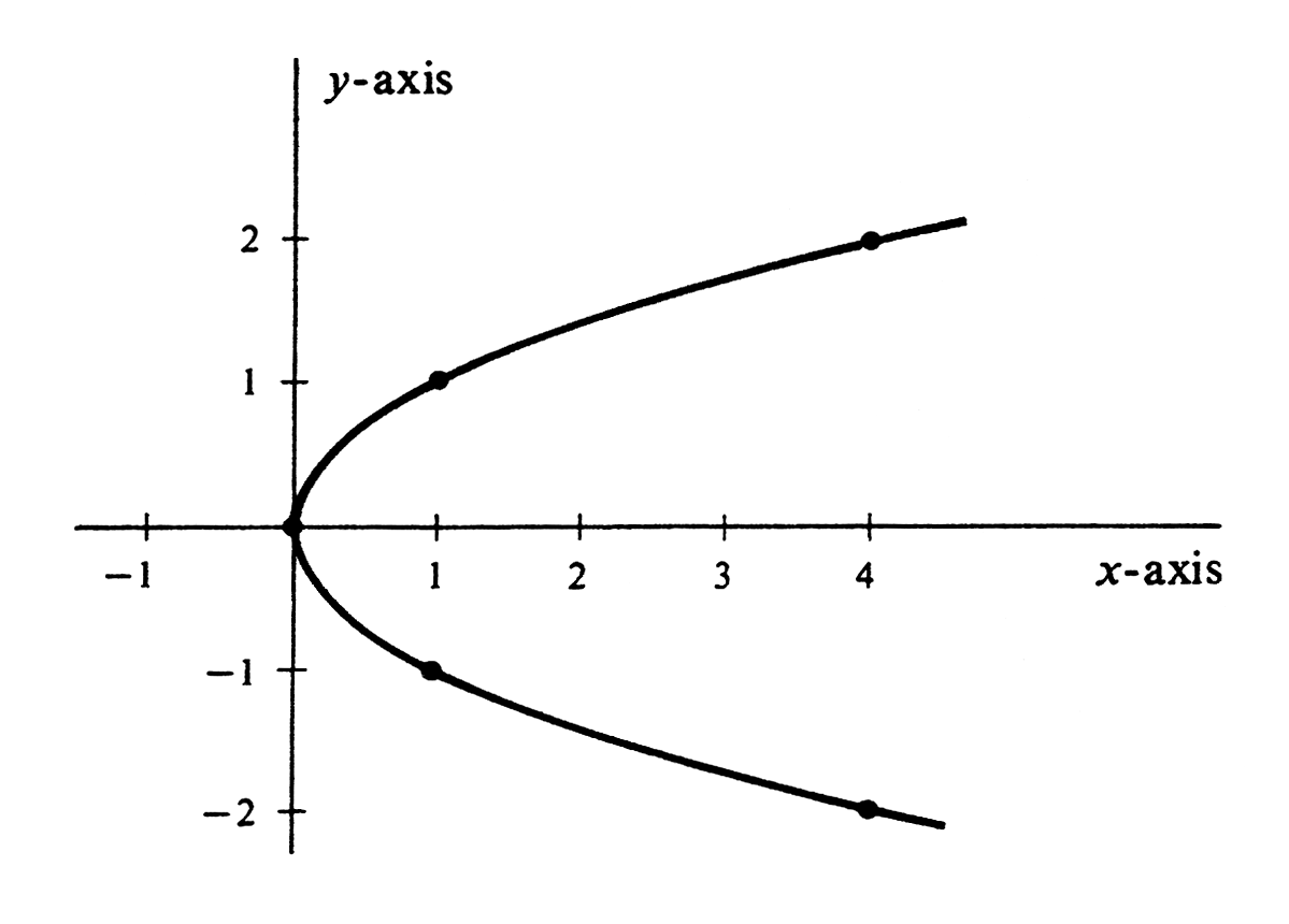
The set of all pairs <math>(x, y)</math> | |||
such that <math>y^2 = x</math> is the curve shown in [[#fig 1.11|Figure]]. | |||
This curve is a parabola, | |||
one of the conic sections, | |||
which are studied in greater detail in Chapter [[guide:56b017bff8#chp 3 |Conic Sections]]. | |||
At present we shall be satisfied with plotting a few points and connecting | |||
them with a smooth curve (see [[#table 1.2 |Table]]). | |||
<div id="fig 1.11" class="d-flex justify-content-center"> | |||
[[File:guide_c5467_scanfig1_11.png | 400px | thumb | ]] | |||
</div> | |||
<span id="table 1.2"/> | |||
{|class="table" | |||
|- | |||
|<math>y</math> || <math>x</math> | |||
|- | |||
|0 || 0 | |||
|- | |||
|<math>\pm1</math> || 1 | |||
|- | |||
|<math>\pm2</math> || 4 | |||
|} | |||
A '''function''' <math>f</math> is any set <math>f</math> of ordered pairs | |||
such that whenever <math>(a, b)</math> and <math>(a, c)</math> belong to <math>f</math>, | |||
then <math>b = c</math>. | |||
Note that every subset of the <math>xy</math>-plane is a set of ordered pairs, | |||
but not every subset is a function. | |||
In particular, the parabola in [[#exam 1.2.4 |Example]] is not, | |||
because it contains both (4, 2) and <math>(4, -2)</math>. | |||
On the other hand, | |||
the straight line in [[#exam 1.2.3 |Example]] is a function. | |||
This condition that a function | |||
must never contain two pairs <math>(a, b)</math> and <math>(a, c)</math> with <math>b \neq c</math> | |||
means geometrically that a subset of the <math>xy</math>-plane is a function | |||
if and only if it never intersects a line parallel to the <math>y</math>-axis | |||
in more than one point. | |||
Hence it is an easy matter to decide which of the following sets | |||
are functions and which are not: | |||
(i) The set <math>f</math> of all pairs <math>(x, y)</math> such that <math>y = x + 1</math>. | |||
(ii) The set <math>g</math> of all pairs <math>(x, y)</math> such that <math>x^2 + y^2 = 1</math>. | |||
(iii) The set <math>F</math> of all pairs <math>(x, y)</math> such that <math>y = x^2 + 2x + 2</math>. | |||
(iv) The set <math>h</math> of all pairs <math>(x, y)</math> such that <math>2x + 3y = 1</math>. | |||
(v) The set <math>G</math> of all pairs <math>(x, y)</math> such that <math>y = \sqrt {x + 2}</math>. | |||
(vi) The set <math>H</math> of all pairs <math>(x, y)</math> such that <math>y^4 = x</math>. | |||
The sets <math>f</math>, <math>F</math>, <math>h</math>, and <math>G</math> are functions, | |||
but <math>g</math> and <math>H</math> are not. | |||
The '''domain''' of a function <math>f</math> is the set of all elements <math>a</math> | |||
for which there is a corresponding <math>b</math> | |||
such that <math>(a, b)</math> belongs to <math>f</math>. | |||
Analogously, the '''range''' of <math>f</math> is the set of all elements <math>b</math> | |||
for which there is an <math>a</math> | |||
such that <math>(a, b)</math> belongs to <math>f</math>. | |||
In (i), | |||
the domain of <math>f</math> is the set <math>\R</math> of all real numbers and so is the range. | |||
On the other hand, in (iii), | |||
although the domain of <math>F</math> is equal to <math>\R</math>, | |||
the range is the interval consisting of all real numbers <math>y \geq 1</math>, | |||
because we can write <math>x^2 + 2x + 2 = (x + 1)^2 + 1 \geq 1</math>. | |||
If a pair <math>(a, b)</math> belongs to a function <math>f</math>, | |||
we call <math>b</math> the '''value of <math>f</math> at <math>a</math>''' and write <math>b = f(a)</math>. | |||
Note that the meaning of <math>f(a)</math> is unambiguous | |||
only because the definition of a function | |||
forbids having <math>(a, b)</math> and <math>(a, c)</math> both belong to <math>f</math> if <math>b \neq c</math>. | |||
Therefore the second member of any ordered pair that belongs to <math>f</math> | |||
is determined by the first member. | |||
<span id="exam 1.2.5"/> | |||
'''Example''' | |||
In (i), | |||
<math display="block"> | |||
\begin{array}{ll} | |||
f(x) = x + 1, &f(a) = a + 1, \\ | |||
f(0) = 1, &f(3 + 4) = (3 + 4) + 1 = 8, \\ | |||
f(-1) = -1 + 1 = 0, &f(a + b) = a + b + 1 . | |||
\end{array} | |||
</math> | |||
In (v), | |||
<math display="block"> | |||
\begin{array}{ll} | |||
G(x) = \sqrt{x + 2}, &G(2x + y) = \sqrt{2x + y + 2}, \\ | |||
G(0) = \sqrt2, &G(-2) = 0, \\ | |||
G(2) = 2, &G(-3) \mbox{is not defined} . | |||
\end{array} | |||
</math> | |||
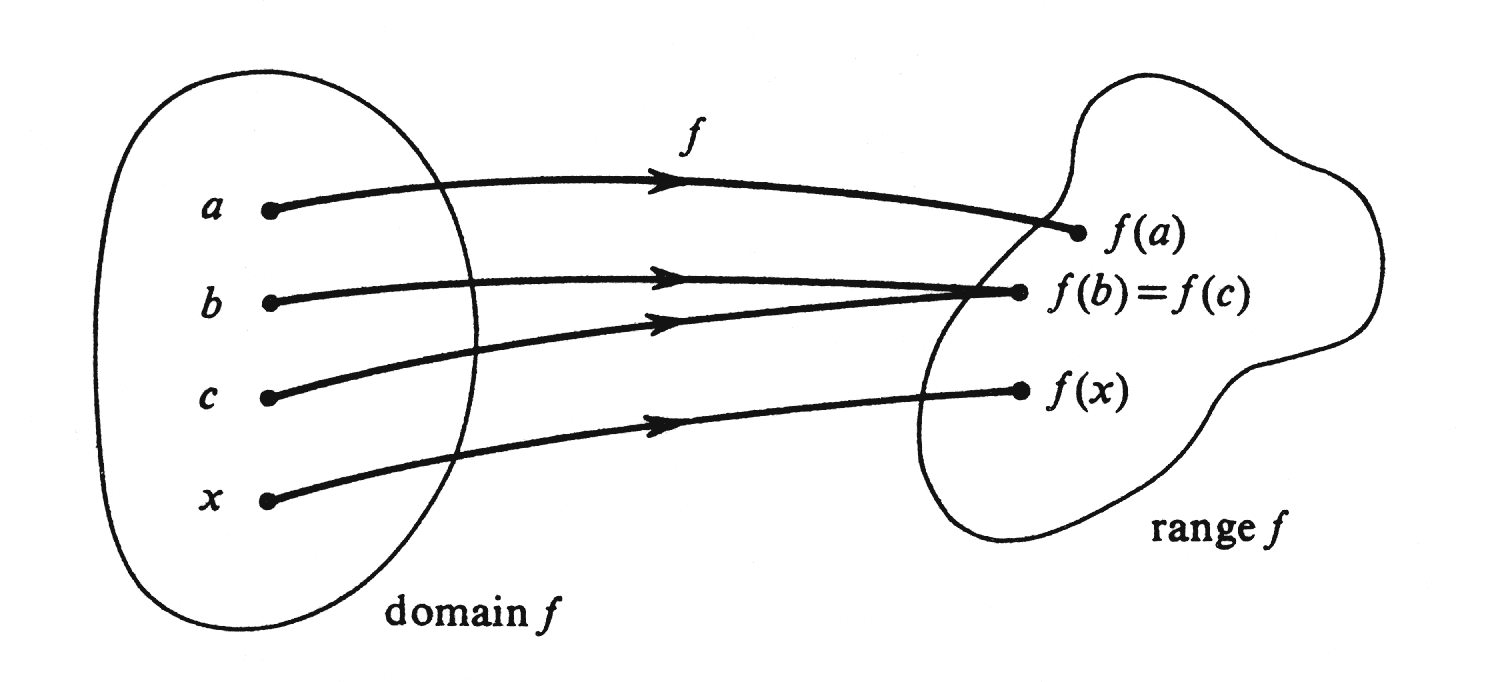
To each element <math>a</math> in the domain of a function <math>f</math> | |||
there corresponds a value <math>f(a)</math> in the range. | |||
This correspondence between domain and range, | |||
which is pictured in [[#fig 1.12|Figure]], | |||
<div id="fig 1.12" class="d-flex justify-content-center"> | |||
[[File:guide_c5467_scanfig1_12.png | 400px | thumb | ]] | |||
</div> | |||
is the central idea in the definition of a function. | |||
Thus the function <math>f</math> that consists of all ordered pairs <math>(x, y)</math> | |||
such that <math>y = x^2</math> and <math>-1 \leq x \leq 2</math> | |||
is interpreted as the rule of correspondence | |||
which assigns to each number in the interval <math>[-1, 2]</math> its square. | |||
We can describe <math>f</math> completely and simply by writing | |||
<math display="block"> | |||
f(x) = x^2, \;\;\; -1 \leq x \leq 2. | |||
</math> | |||
Examples of other functions are | |||
<math display="block"> | |||
g(x) = \sqrt{x - 1}, \prov{-1 \leq x < \infty}, | |||
</math> | |||
<math display="block"> | |||
F(x) = x^2, \prov{-\infty < x < \infty,} | |||
</math> | |||
<math display="block"> | |||
h(x) = \frac{x}{x + 2}, \prov{x \neq -2} . | |||
</math> | |||
Note that the functions <math>f</math> and <math>F</math> immediately above | |||
are ''not'' equal, | |||
although <math>f</math> is a subset of <math>F</math>. | |||
Two functions are equal | |||
if they are one and the same set of ordered pairs. | |||
It follows that | |||
{{proofcard|Proposition|thm_1.2.4|Functions <math>f</math> and <math>g</math> are equal | |||
if and only if they have the same domain <math>D</math> | |||
and <math>f(x) = g(x)</math> for every element <math>x</math> in <math>D</math>.|}} | |||
Thus any complete description of a function | |||
must include a description of its domain. | |||
Sometimes this information is in fact omitted. | |||
We shall adopt the convention that | |||
if no explicit description of the domain of a function is given, | |||
then its domain is assumed to be the largest set of real numbers | |||
that makes sense. | |||
For example, the domain of the function <math>H</math> defined by | |||
<math display="block"> | |||
H(x) = \frac{1}{x^2 - x - 2} = \frac{1}{(x + 1)(x - 2)} | |||
</math> | |||
is assumed to be the entire set of real numbers | |||
with the exception of <math>-1</math> and 2. | |||
It is sometimes helpful to think of a function | |||
as a computing machine. | |||
Imagine a computing machine, | |||
named <math>f</math>, | |||
which is provided with an input tape, | |||
an output tape, | |||
and a button (see [[#fig 1.13|Figure]]). | |||
<div id="fig 1.13" class="d-flex justify-content-center"> | |||
[[File:guide_c5467_scanfig1_13.png | 400px | thumb | ]] | |||
</div> | |||
One writes a number <math>x</math> on the input tape | |||
and pushes the button. | |||
If <math>x</math> is one of the inputs which the machine will accept, | |||
i.e., if <math>x</math> is in the domain of <math>f</math>, | |||
the machine whirs contentedly and prints an output, | |||
which we denote <math>f(x)</math>, | |||
on the output tape. | |||
If <math>x</math> is not in the prescribed domain, | |||
either nothing happens or a red light flashes. | |||
We have already seen that | |||
one of the best ways of describing a subset of <math>\R^2</math> | |||
is to draw a picture of it. | |||
If this subset happens to be a function, | |||
we call the picture the graph of the function. | |||
More specifically, | |||
if a function <math>f</math> is a subset of <math>\R^2</math>, | |||
its '''graph''' is the set of all points in the plane | |||
that correspond to ordered pairs of the form <math>(x, f(x))</math>. | |||
Note that the graph of <math>f</math> | |||
depends on the correspondence between ordered pairs and points; | |||
i.e., it depends on the choice of axes. | |||
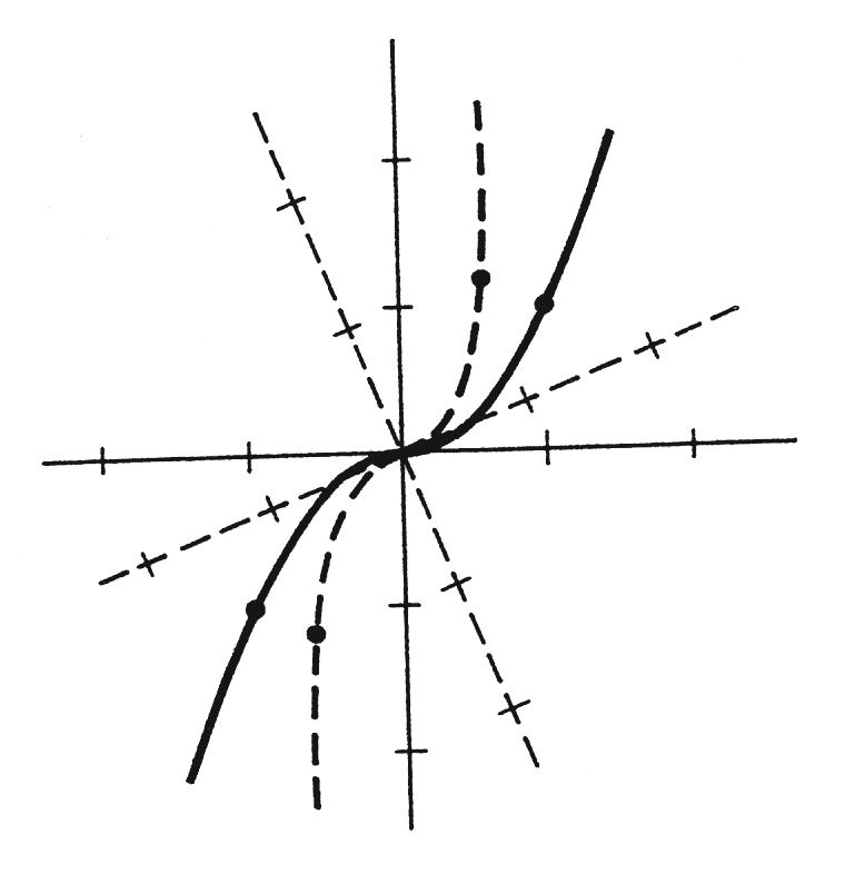
To illustrate this, | |||
in [[#fig 1.14|Figure]] | |||
<div id="fig 1.14" class="d-flex justify-content-center"> | |||
[[File:guide_c5467_scanfig1_14.png | 400px | thumb | ]] | |||
</div> | |||
we have drawn the graph of the function <math>f</math> | |||
defined by <math>f(x) = x^3</math> | |||
for two sets of axes. | |||
For a single choice of axes, | |||
we simply identify ordered pairs and points, | |||
and under this identification | |||
a function and its graph become the same thing. | |||
Most of the functions encountered in an introduction to calculus | |||
are defined by means of a single equation; | |||
e.g., <math>h(x) = x^3 + 3</math>. | |||
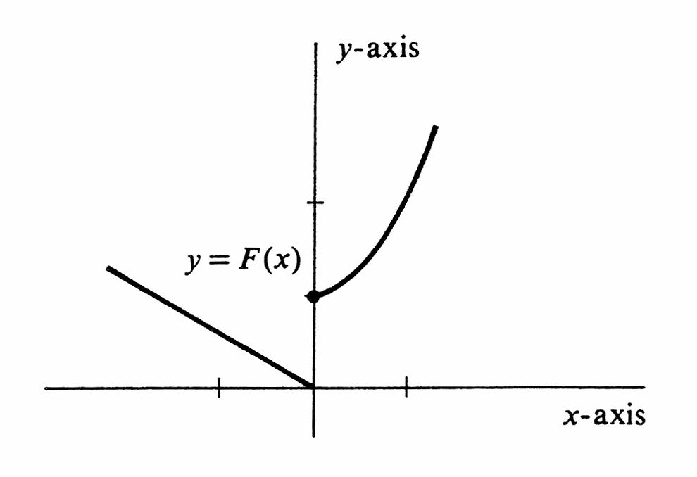
It is a bad mistake, however, to assume that this is always true. The function <math>F</math> given by | |||
<math display="block"> | |||
F(x) = \left \{ \begin{array}{ll} | |||
x^2 + 1 &\mbox{if $x \geq 0$},\\ | |||
-\frac{x}{2} &\mbox{if $x < 0$}, | |||
\end{array} | |||
\right. | |||
</math> | |||
requires two equations for its definition. The graph of <math>F</math> is shown in [[#fig 1.15|Figure]]. | |||
<div id="fig 1.15" class="d-flex justify-content-center"> | |||
[[File:guide_c5467_scanfig1_15.png | 400px | thumb | ]] | |||
</div> | |||
Another function, which is so wild that it is impossible to draw its graph, is the following: | |||
<math display="block"> | |||
g(x) = \left \{ \begin{array}{ll} | |||
0 & \mbox{if $x$ is rational,}\\ | |||
1 & \mbox{if $x$ is irrational.} \end{array} | |||
\right. | |||
</math> | |||
The ordered pairs that comprise a function | |||
are not necessarily pairs of numbers. | |||
An example is the function, | |||
mentioned earlier in this section, | |||
which assigns to each triangle | |||
the point of intersection of its medians. | |||
It is possible for the domain of a function to be | |||
a set of ordered pairs. | |||
Consider the function <math>f</math> consisting of all ordered pairs <math>((x, y), z)</math>, | |||
where <math>x, y</math>, and <math>z</math> are numbers that satisfy | |||
<math>x \geq y</math> and <math>z = 2x^2 + y^2</math>. | |||
We describe this function simply as follows: | |||
<span id{{=}}"eq1.2.4"/> | |||
<math display="block"> | |||
\begin{equation} | |||
f(x, y) = 2x^2 + y^2, \;\;\; x \geq y. | |||
\label{eq1.2.4} | |||
\end{equation} | |||
</math> | |||
As a final example of a function, | |||
consider the rule of correspondence that assigns to each person | |||
his or her male parent. | |||
As we have indicated, | |||
the definition of a function is appallingly general. | |||
One of our tasks is to delineate properly | |||
the kinds of functions studied in calculus. | |||
To begin with, | |||
a function <math>f</math> is said to be '''real-valued''' | |||
if its range is a subset of <math>\R</math>, the set of real numbers. | |||
If the domain of <math>f</math> is a subset of <math>\R</math>, | |||
we call <math>f</math> a '''function of a real variable'''. | |||
The function <math>f(x, y)</math> defined [[#eq1.2.4 |in]] | |||
has as its domain a subset of <math>\R^2</math>. | |||
It is a real-valued function of two real variables. | |||
For the most part, | |||
a first course in calculus is a study of | |||
real-valued functions of one real variable. | |||
==General references== | |||
{{cite web |title=Crowell and Slesnick’s Calculus with Analytic Geometry|url=https://math.dartmouth.edu/~doyle/docs/calc/calc.pdf |last=Doyle |first=Peter G.|date=2008 |access-date=Oct 29, 2024}} | |||
Latest revision as of 23:08, 3 November 2024
The set whose members consist of just the two elements [math]a[/math] and [math]b[/math]
is denoted [math]\{ a, b \}[/math].
The notation is not perfect because it suggests that the members [math]a[/math] and [math]b[/math] have been ordered:
[math]a[/math] is written first and [math]b[/math] second. Actually no ordering is present because [math]\{ a, b \} = \{ b, a \}[/math]. Note also that if [math]a = b[/math], then [math]\{ a, b \} = \{ b, a \} = \{ a \}[/math]. It can happen, however, that the ingredient of order is essential. We therefore introduce the notion of an ordered pair [math](a, b)[/math] whose first member is [math]a[/math] and whose second member is [math]b[/math]. The characteristic property of ordered pairs is
In particular [math](a, b) = (b, a)[/math] if and only if [math]a = b[/math]. In Section \secref{1.1} we saw that the set [math]\R[/math] of all real numbers can be thought of as a straight line. We shall now show that every ordered pair [math](a, b)[/math] of real numbers [math]a[/math] and [math]b[/math] can be identified with a point in a plane. This brings up a notational problem: Is [math](5, 7)[/math] the ordered pair of real numbers or is it the open interval consisting of all [math]x[/math] such that [math]5 \lt x \lt 7[/math]? The answer is that it is impossible to tell out of context---just as it is impossible to tell whether the word “well” is the noun or the adverb. Consider two distinct real number lines drawn in a plane so that they intersect at the number [math]0[/math] on each line. One of the lines is traditionally drawn horizontal and called the [math]x[/math]-axis, and the other is made perpendicular to it and called the [math]y[/math]-axis. The orientation is chosen so that the number [math]1[/math] on the [math]x[/math]-axis lies to the right of [math]0[/math], and the number [math]1[/math] on the [math]y[/math]-axis is above [math]0[/math]. It is also customary to use the same scale of distances on both axes. For every ordered pair [math](a, b)[/math] of real numbers, let [math]L_a[/math] be the line parallel to the [math]y[/math]-axis that cuts the [math]x[/math]-axis at [math]a[/math], and let [math]M_b[/math] be the line parallel to the [math]x[/math]-axis that cuts the [math]y[/math]-axis at [math]b[/math]. We assign the point of intersection of [math]L_a[/math] and [math]M_b[/math] to the ordered pair [math](a, b)[/math] (see Figure). The numbers [math]a[/math] and [math]b[/math] are called the coordinates of the point. [math]a[/math] is the [math]x[/math]-coordinate (or abscissa) and [math]b[/math] is the [math]y[/math]-coordinate (or ordinate).
If the pairs [math](a, b)[/math] and [math](c, d)[/math] are not equal, then the points in the plane assigned to them will be different. In addition, every point in the plane has a number pair assigned to it: Starting with a point, draw the two lines through it which are parallel to the [math]x[/math]-axis and the [math]y[/math]-axis. One line cuts the [math]x[/math]-axis at a number [math]a[/math], and the other cuts the [math]y[/math]-axis at [math]b[/math]. The ordered pair [math](a, b)[/math] has the original point assigned to it. It follows that our assignment
is a one-to-one correspondence between the set of all ordered pairs of real numbers, which we denote by [math]\R^2[/math], and the set of all points of the plane. It is convenient simply to identify [math]\R^2[/math] with the plane together with the two axes.
Example
Plot the points
[math](1, 2), (-2, 3), (0, 1), (4, 0), (-2, -3)[/math], and [math](2, -3)[/math]
on the [math]xy[/math]-plane
(see Figure).
The usefulness of the idea of an ordered pair is by no means limited to pairs of real numbers. In plane geometry, for example, we may consider the set of all ordered pairs [math](T, p)[/math] in which [math]T[/math] is a triangle and [math]p[/math] is the point of intersection of its medians. In the three-dimensional extension of the [math]xy[/math]-plane, the set [math]\R^3[/math] of all ordered triples [math](a, b, c)[/math] of real numbers is identified with the set of all points in three-dimensional space. The definition of an ordered triple can be reduced to that of an ordered pair by defining [math](a, b, c)[/math] to be [math]((a, b), c)[/math].
Let [math]P = (a, b)[/math] and [math]Q = (c, d)[/math] be arbitrary elements in the set [math]\R^2[/math] of all ordered pairs of real numbers. We define the distance between [math]P[/math] and [math]Q[/math] by the formula
[math]\dist(P, Q) \geq 0[/math]; i.e., distance is never negative.
[math]\dist(P, Q) = 0[/math] if and only if [math]P = Q[/math].
[math]\dist(P, Q) = \dist (Q, P)[/math].
Another consequence of (1) is that it is no longer simply a matter of tradition and convenience that we draw the [math]y[/math]-axis perpendicular to the [math]x[/math]-axis. It follows from consideration of the Pythagorean Theorem and its converse (see Figure) that the above definition of distance between elements of [math]\R^2[/math] corresponds with our geometric notion of the distance between points in the Euclidean plane if and only if the two coordinate axes are perpendicular and the scales are the same on both.
Example
Let [math]C[/math] be the subset of the [math]xy[/math]-plane
consisting of all points whose distance from (1,1) is equal to 2.
Thus [math]C[/math] is the circle shown in Figure.
If [math](x, y)[/math] is an arbitrary point in the [math]xy[/math]-plane,
its distance from [math](1,1)[/math]
is equal to
[math]\sqrt{(x - 1)^2 + (y - 1)^2}[/math].
Hence, [math](x, y)[/math] belongs to [math]C[/math]
if and only if
The set of all points [math](x, y)[/math] in the plane that satisfy a given equation is called the graph of the equation. Hence, in the above example, the circle [math]C[/math] is the graph of the equation [math](x - 1)^2 + (y - 1)^2 = 4[/math]. Example
Let [math]L[/math] be the set of all ordered pairs [math](x, y)[/math] such that [math]y = 2x - 3[/math]. For each real number [math]x[/math], there is one and only one number [math]y[/math] such that [math](x, y)[/math] belongs to [math]L: y = 2x - 3[/math]. To see what [math]L[/math] looks like, we plot five of its points (see Table). As shown in Figure, all these points lie on a straight line. In Section \secref{1.5} we shall justify the natural conjecture that this straight line is the set [math]L[/math].
| [math]x[/math] | [math]y=2x - 3[/math] |
| 0 | -3 |
| 1 | -1 |
| 2 | 1 |
| 3 | 3 |
Example
The set of all pairs [math](x, y)[/math] such that [math]y^2 = x[/math] is the curve shown in Figure. This curve is a parabola, one of the conic sections, which are studied in greater detail in Chapter Conic Sections. At present we shall be satisfied with plotting a few points and connecting them with a smooth curve (see Table).
| [math]y[/math] | [math]x[/math] |
| 0 | 0 |
| [math]\pm1[/math] | 1 |
| [math]\pm2[/math] | 4 |
A function [math]f[/math] is any set [math]f[/math] of ordered pairs such that whenever [math](a, b)[/math] and [math](a, c)[/math] belong to [math]f[/math], then [math]b = c[/math]. Note that every subset of the [math]xy[/math]-plane is a set of ordered pairs, but not every subset is a function. In particular, the parabola in Example is not, because it contains both (4, 2) and [math](4, -2)[/math]. On the other hand, the straight line in Example is a function. This condition that a function must never contain two pairs [math](a, b)[/math] and [math](a, c)[/math] with [math]b \neq c[/math] means geometrically that a subset of the [math]xy[/math]-plane is a function if and only if it never intersects a line parallel to the [math]y[/math]-axis in more than one point. Hence it is an easy matter to decide which of the following sets are functions and which are not: (i) The set [math]f[/math] of all pairs [math](x, y)[/math] such that [math]y = x + 1[/math]. (ii) The set [math]g[/math] of all pairs [math](x, y)[/math] such that [math]x^2 + y^2 = 1[/math]. (iii) The set [math]F[/math] of all pairs [math](x, y)[/math] such that [math]y = x^2 + 2x + 2[/math]. (iv) The set [math]h[/math] of all pairs [math](x, y)[/math] such that [math]2x + 3y = 1[/math]. (v) The set [math]G[/math] of all pairs [math](x, y)[/math] such that [math]y = \sqrt {x + 2}[/math]. (vi) The set [math]H[/math] of all pairs [math](x, y)[/math] such that [math]y^4 = x[/math]. The sets [math]f[/math], [math]F[/math], [math]h[/math], and [math]G[/math] are functions, but [math]g[/math] and [math]H[/math] are not. The domain of a function [math]f[/math] is the set of all elements [math]a[/math] for which there is a corresponding [math]b[/math] such that [math](a, b)[/math] belongs to [math]f[/math]. Analogously, the range of [math]f[/math] is the set of all elements [math]b[/math] for which there is an [math]a[/math] such that [math](a, b)[/math] belongs to [math]f[/math]. In (i), the domain of [math]f[/math] is the set [math]\R[/math] of all real numbers and so is the range. On the other hand, in (iii), although the domain of [math]F[/math] is equal to [math]\R[/math], the range is the interval consisting of all real numbers [math]y \geq 1[/math], because we can write [math]x^2 + 2x + 2 = (x + 1)^2 + 1 \geq 1[/math]. If a pair [math](a, b)[/math] belongs to a function [math]f[/math], we call [math]b[/math] the value of [math]f[/math] at [math]a[/math] and write [math]b = f(a)[/math]. Note that the meaning of [math]f(a)[/math] is unambiguous only because the definition of a function forbids having [math](a, b)[/math] and [math](a, c)[/math] both belong to [math]f[/math] if [math]b \neq c[/math]. Therefore the second member of any ordered pair that belongs to [math]f[/math] is determined by the first member.
Example
In (i),
To each element [math]a[/math] in the domain of a function [math]f[/math] there corresponds a value [math]f(a)[/math] in the range. This correspondence between domain and range, which is pictured in Figure,
is the central idea in the definition of a function. Thus the function [math]f[/math] that consists of all ordered pairs [math](x, y)[/math] such that [math]y = x^2[/math] and [math]-1 \leq x \leq 2[/math] is interpreted as the rule of correspondence which assigns to each number in the interval [math][-1, 2][/math] its square. We can describe [math]f[/math] completely and simply by writing
Functions [math]f[/math] and [math]g[/math] are equal if and only if they have the same domain [math]D[/math] and [math]f(x) = g(x)[/math] for every element [math]x[/math] in [math]D[/math].
Thus any complete description of a function must include a description of its domain. Sometimes this information is in fact omitted. We shall adopt the convention that if no explicit description of the domain of a function is given, then its domain is assumed to be the largest set of real numbers that makes sense. For example, the domain of the function [math]H[/math] defined by
One writes a number [math]x[/math] on the input tape and pushes the button. If [math]x[/math] is one of the inputs which the machine will accept, i.e., if [math]x[/math] is in the domain of [math]f[/math], the machine whirs contentedly and prints an output, which we denote [math]f(x)[/math], on the output tape. If [math]x[/math] is not in the prescribed domain, either nothing happens or a red light flashes. We have already seen that one of the best ways of describing a subset of [math]\R^2[/math] is to draw a picture of it. If this subset happens to be a function, we call the picture the graph of the function. More specifically, if a function [math]f[/math] is a subset of [math]\R^2[/math], its graph is the set of all points in the plane that correspond to ordered pairs of the form [math](x, f(x))[/math]. Note that the graph of [math]f[/math] depends on the correspondence between ordered pairs and points; i.e., it depends on the choice of axes. To illustrate this, in Figure
we have drawn the graph of the function [math]f[/math] defined by [math]f(x) = x^3[/math] for two sets of axes. For a single choice of axes, we simply identify ordered pairs and points, and under this identification a function and its graph become the same thing. Most of the functions encountered in an introduction to calculus are defined by means of a single equation; e.g., [math]h(x) = x^3 + 3[/math]. It is a bad mistake, however, to assume that this is always true. The function [math]F[/math] given by
requires two equations for its definition. The graph of [math]F[/math] is shown in Figure.
Another function, which is so wild that it is impossible to draw its graph, is the following:
General references
Doyle, Peter G. (2008). "Crowell and Slesnick's Calculus with Analytic Geometry" (PDF). Retrieved Oct 29, 2024.
