guide:D0085fde68

[math] \newcommand{\ex}[1]{\item } \newcommand{\sx}{\item} \newcommand{\x}{\sx} \newcommand{\sxlab}[1]{} \newcommand{\xlab}{\sxlab} \newcommand{\prov}[1] {\quad #1} \newcommand{\provx}[1] {\quad \mbox{#1}} \newcommand{\intext}[1]{\quad \mbox{#1} \quad} \newcommand{\R}{\mathrm{\bf R}} \newcommand{\Q}{\mathrm{\bf Q}} \newcommand{\Z}{\mathrm{\bf Z}} \newcommand{\C}{\mathrm{\bf C}} \newcommand{\dt}{\textbf} \newcommand{\goesto}{\rightarrow} \newcommand{\ddxof}[1]{\frac{d #1}{d x}} \newcommand{\ddx}{\frac{d}{dx}} \newcommand{\ddt}{\frac{d}{dt}} \newcommand{\dydx}{\ddxof y} \newcommand{\nxder}[3]{\frac{d^{#1}{#2}}{d{#3}^{#1}}} \newcommand{\deriv}[2]{\frac{d^{#1}{#2}}{dx^{#1}}} \newcommand{\dist}{\mathrm{distance}} \newcommand{\arccot}{\mathrm{arccot\:}} \newcommand{\arccsc}{\mathrm{arccsc\:}} \newcommand{\arcsec}{\mathrm{arcsec\:}} \newcommand{\arctanh}{\mathrm{arctanh\:}} \newcommand{\arcsinh}{\mathrm{arcsinh\:}} \newcommand{\arccosh}{\mathrm{arccosh\:}} \newcommand{\sech}{\mathrm{sech\:}} \newcommand{\csch}{\mathrm{csch\:}} \newcommand{\conj}[1]{\overline{#1}} \newcommand{\mathds}{\mathbb} [/math]

If [math]f[/math] and [math]g[/math] are two functions, a new function [math]f(g)[/math], called the composition of [math]g[/math] with [math]f[/math], is defined by

[[math]] (f(g))(x) = f(g(x)). [[/math]]

For example, if [math]f(x) = x^3 - 1[/math] and [math]g(x) = \frac{x + 1}{x - 1}[/math], then

[[math]] \begin{eqnarray} \label{eq1.3.1} (f(g))(x) &=& f(g(x)) = (g(x))^3 - 1 \\ &=& \biggl( \frac{x + 1}{x - 1}\biggr)^3 - 1 = \frac{2(3x^2 + 1)}{(x - 1)^3} . \end{eqnarray} [[/math]]

The composition of two functions is the function obtained by applying one after the other. If [math]f[/math] and [math]g[/math] are regarded as computing machines, then [math]f(g)[/math] is the composite machine constructed by feeding the output of [math]g[/math] into the input of [math]f[/math] as indicated in Figure.

In general it is not true that [math]f(g) = g(f)[/math]. In the above example we have

[[math]] \begin{eqnarray} \label{eq1.3.2} (g(f))(x) &=& g(f(x)) = \frac{f(x) + 1}{f(x) - 1} \\ &=& \frac{(x^3 - 1) + 1}{(x^3 - 1) - 1} = \frac{x^3}{x^3 - 2} , \end{eqnarray} [[/math]]

and the two functions are certainly not the same. In terms of ordered pairs the composition [math]f(g)[/math] of [math]g[/math] with [math]f[/math] is formally defined to be the set of all ordered pairs [math](a, c)[/math] for which there is an element [math]b[/math] such that [math]b = g(a)[/math] and [math]c = f(b)[/math]. If [math]f[/math] and [math]g[/math] are two real-valued functions, we can perform the usual arithmetic operations of addition, subtraction, multiplication, and division. Thus for the functions [math]f(x) = x^3 - 1[/math] and [math]g(x) = \frac{x + 1}{x - 1}[/math], we have

[[math]] \begin{eqnarray*} f(x) + g(x) &=& x^3 - 1 + \frac{x + 1}{x - 1} , \\ f(x) - g(x) &=& x^3 - 1 - \frac{x + 1}{x - 1} , \\ f(x)g(x) &=& (x^3 -1) \frac{x + 1}{x - 1} , \\ &=& (x^2 + x + 1)(x + 1) \provx{if $x \neq 1$}, \\ f(x)/g(x) &=& \frac{x^3 - 1}{\frac{x + 1}{x - 1}} \\ &=& \frac{(x^3 - 1)(x - 1)}{x + 1}. \end{eqnarray*} [[/math]]

Just as with the composition of two functions, each arithmetic operation provides a method of constructing a new function from the two given functions [math]f[/math] and [math]g[/math]. The natural notations for these new functions are [math]f + g[/math], [math]f - g[/math], [math]fg[/math], and [math]\frac{f}{g}[/math]. They are defined by the formulas

[[math]] \begin{eqnarray*} (f + g)(x) &=& f(x) + g(x), \\ (f - g)(x) &=& f(x) - g(x), \\ (fg)(x) &=& f(x)g(x), \\ {\frac{f}{g}}(x) &=& \frac{f(x)}{g(x)} \provx{if $g(x) \neq 0$}. \end{eqnarray*} [[/math]]

The product function [math]fg[/math] should not be confused with the composite function [math]f(g)[/math]. For example, if [math]f(x) = x^5[/math] and [math]g(x) = x^3[/math], then we have [math](fg)(x) = f(x)g(x) = {x^5} \cdot {x^3} = x^8[/math], whereas

[[math]] (f(g))(x) = f(g(x)) = (x^3)^5 = x^{15}. [[/math]]

We may also form the product [math]af[/math] of an arbitrary real number [math]a[/math] and real-valued function [math]f[/math]. The product function is defined by

[[math]] (af)(x)= af(x). [[/math]]

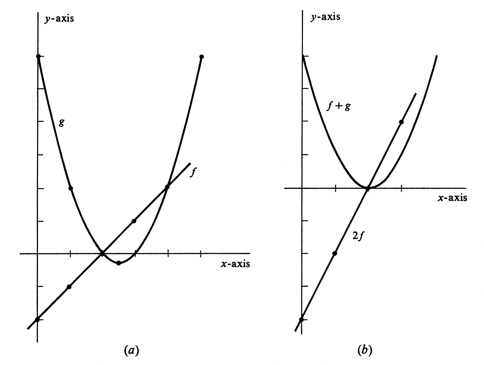
Example \label{exam 1.3.1} Let functions [math]f[/math] and [math]g[/math] be defined by [math]f(x) = x - 2[/math] and [math]g(x) = x^2 - 5x + 6[/math]. Draw the graphs of [math]f[/math], [math]g[/math], [math]2f[/math], and [math]f + g[/math]. We compute the function values corresponding to several different numbers [math]x[/math] in table and table. The resulting graphs of [math]f[/math] and [math]g[/math] are, respectively, the straight line and parabola shown in Figure(a).

It turns out that the graphs of [math]2f[/math] and [math]f + g[/math] are also a straight line and a parabola. They are drawn in Figure(b). To see why the graph of [math]f + g[/math] is a parabola, observe that

[[math]] \begin{eqnarray*} (f + g)(x) &=& f(x) + g(x) = (x - 2) + (x^2 - 5x + 6) = x^2 - 4x + 4 \\ &=& (x - 2)^2. \end{eqnarray*} [[/math]]

It follows that [math]f + g[/math] is very much like the function defined by [math]y = x^2[/math]. Instead of simply squaring a number, [math]f + g[/math] first subtracts [math]2[/math] and then squares. Its graph will be just like that of [math]y = x^2[/math] except that it will be shifted two units to the right.

[[math]] \begin{array}{r|r|c} \hline x & f(x) & 2f(x) \\ \hline 0 & -2 & -4 \\ 1 & -1 & -2 \\ 2 & 0 & 0 \\ 3 & 1 & 2 \\ \hline \end{array} [[/math]]

[[math]] \begin{array}{r|c} \hline x & g(x) \\ \hline 0 & 6 \\ 5 & 6 \\ \frac{5}{2} & -\frac{1}{4} \\ 1 & 2 \\ 4 & 2 \\ \hline \end{array} [[/math]]

Up to this point we have used the letters [math]f[/math], [math]g[/math], [math]h[/math], [math]F[/math], [math]G[/math], and [math]H[/math] to denote functions,and the letters [math]x[/math], [math]y[/math], [math]a[/math], [math]b[/math], and [math]c[/math] to denote elements of sets---usually real numbers. However, the letters in the second set are sometimes also used as functions. This occurs, for example, when we speak of [math]x[/math] as a real variable. As such, it not only is the name of a real number but also can take on many different values: [math]5[/math], or [math]-7[/math], or [math]\pi[/math], or \ldots. Thus the variable [math]x[/math] is a function. Specifically, it is the very simple function that assigns the value [math]5[/math] to the number [math]5[/math], the value [math]-7[/math] to the number [math]-7[/math], the value [math]\pi[/math] to [math]\pi[/math], \ldots. For every real number [math]a[/math], we have

[[math]] x(a) = a. [[/math]]

This function is called the identity function. Suppose, for example, that [math]s[/math] is used to denote the distance that a stone falling freely in space has fallen. The value of [math]s[/math] increases as the stone falls and depends on the length of time [math]t[/math] that it has fallen according to the equation [math]s= {\frac{1}{2}}g{t^2}[/math], where [math]g[/math] is the constant gravitational acceleration. (This formula assumes no air resistance, that the stone was at rest at time [math]t = 0[/math], and that distance is measured from the starting point.) Thus [math]s[/math] has the value [math]{\frac{9}{2}}g[/math] if [math]t[/math] has the value [math]3[/math], and, more generally, the value [math]{\frac{1}{2}}g{a^2}[/math] when [math]t[/math] has the value [math]a[/math]. If we consider [math]t[/math] to be another name for the identity function, then [math]s[/math] may be regarded as the function whose value is

[[math]] s(a) = {\frac{1}{2}}{g{a^2}} = {\frac{1}{2}}{g(t(a))^2} [[/math]]

for every real number [math]a[/math]. The original equation [math]s = {\frac{1}{2}}g{t^2}[/math] then states the relation between the two functions [math]s[/math] and [math]t[/math]. The fact that [math]s[/math] and [math]t[/math] take on different values is also expressed by referring to them as variables. A variable is simply a name of a function. In our example [math]s[/math] is called a dependent variable, and [math]t[/math] an independent variable, because the values of [math]s[/math] depend on those of [math]t[/math] according to [math]s = {\frac{1}{2}}g{t^2}[/math]. Thus an independent variable is a name for the identity function, and a dependent variable is one that is not independent. A real variable is therefore a name of a real-valued function. Since the arithmetic operations of addition, subtraction, multiplication, and division have been defined for real-valued functions, they are automatically defined for real variables. We shall generally use the letter [math]x[/math] to denote an independent variable. This raises the question: How does one tell whether an occurrence of [math]x[/math] denotes a real number or the identity function? The answer is that the notation alone does not tell, but the context and the reader's understanding should. However, a more practical reply is that it doesn't really make much difference. We may regard [math]f(x)[/math] as either the value of the function [math]f[/math] at the number [math]x[/math] or as the composition of [math]f[/math] with the variable [math]x[/math]. If [math]x[/math] is an independent variable, the function [math]f(x)[/math] is then the same thing as [math]f[/math].

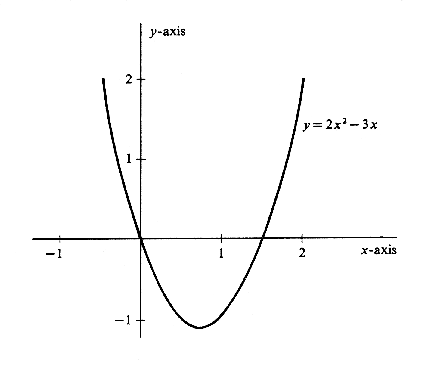
Example \label{exam 1.3.2} The conventions that we have adopted concerning the use of variables give our notations a flexibility that is both consistent and extremely useful. Consider, for example, the equation

[[math]] y= 2x^2 - 3x. [[/math]]

On the one hand, we may consider the subset of [math]\R^2[/math], pictured in Figure,

that consists of all ordered pairs [math](x, y)[/math] such that [math]y = 2x^2 - 3x[/math]. This subset is a function [math]f[/math] whose value at an arbitrary real number [math]x[/math] is the real number [math]f(x) = 2x^2 - 3x[/math]. Alternatively, we may regard [math]x[/math] as an independent variable, i.e., the identity function. The composition of [math]f[/math] with [math]x[/math] is then the function [math]f(x) = 2x^2 - 3x[/math], whose value at [math]2[/math], for instance, is

[[math]] (f(x))(2) = f(x(2)) = f(2) = 8 - 6 = 2. [[/math]]

A third interpretation is that [math]y[/math] is a dependent variable that depends on [math]x[/math] according to the equation [math]y = 2x^2 - 3x[/math]. That is, [math]y[/math] is the name of the function [math]2x^2 - 3x[/math].

Example \label{exam 1.3.3} Let [math]F[/math] be the function defined by [math]F(x) = x^3 + x + 1[/math]. If [math]u = \sqrt{x - 2}[/math], then

[[math]] \begin{eqnarray*} F(u) &=& u^3 + u + 1 \\ &=& (x - 2)^{3/2} + (x - 2)^{1/2} + 1. \end{eqnarray*} [[/math]]

If we denote the function [math]F(x)[/math] by [math]w[/math], then

[[math]] u + w = \sqrt{x - 2} + x^3 + x + 1, [[/math]]

[[math]] uw = (x - 2)^{1/2} (x^3 + x + 1). [[/math]]

On the other hand, we may let [math]G[/math] be the function defined by [math]G(x) = \sqrt{x - 2}[/math] for every real number [math]x \geq 2[/math]. Then [math]G + F[/math] and [math]GF[/math] are the functions defined, respectively, by

[[math]] \begin{eqnarray*} (G + F)(x) &=& G(x) + F(x) \\ &=& \sqrt{x - 2} + x^3 + x + 1, \\ (GF)(x) &=& G(x)F(x) \\ &=& (x - 2)^{1/2} (x^3 + x + 1). \end{eqnarray*} [[/math]]

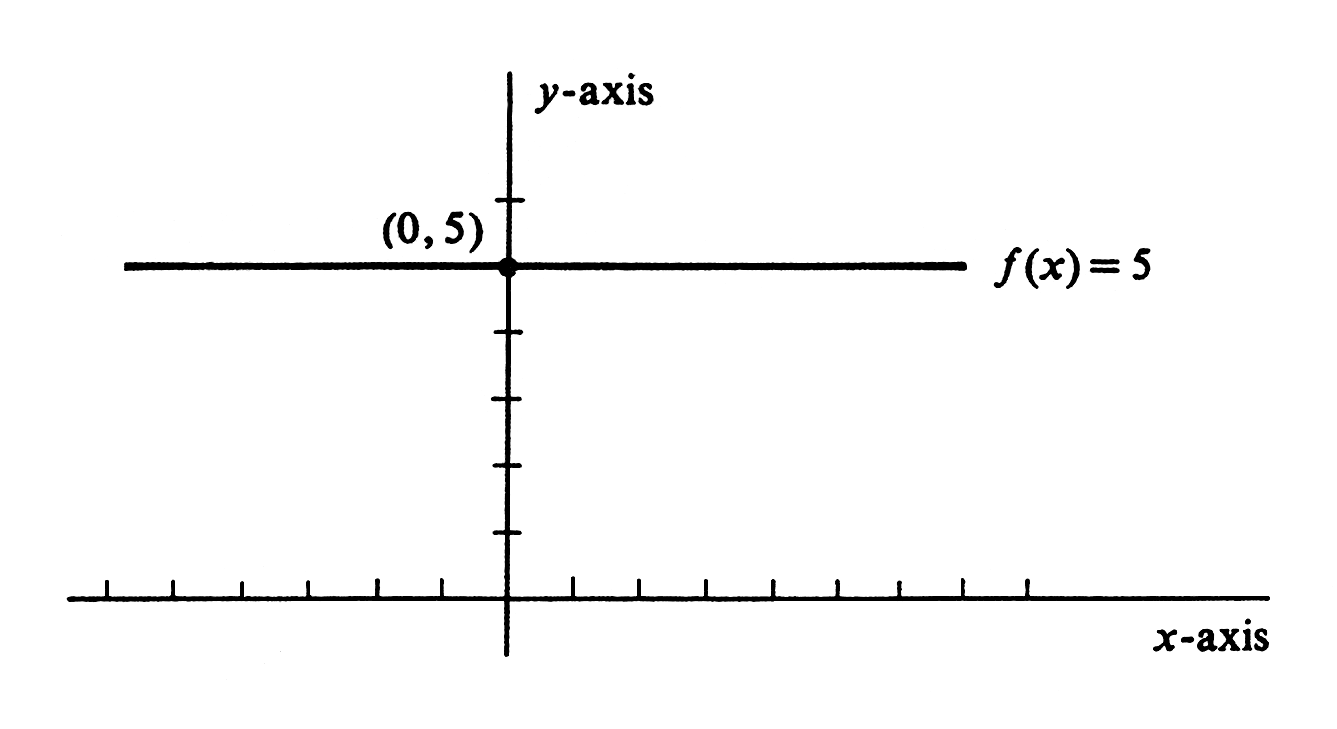
To say that [math]a[/math] is a real constant means first that it is a real number. Second, it may or may not matter which real number [math]a[/math] is, but it is fixed for the duration of the discussion in which it occurs. Similarly, a constant function is one which takes on just one value; i.e., its range consists of a single element. For example, consider the constant function [math]f[/math] defined by

[[math]] f(x) = 5, \;\;\; - \infty \lt x \lt \infty. [[/math]]

The graph of [math]f[/math] is the straight line parallel to the [math]x[/math]-axis that intersects the [math]y[/math]-axis in the point (0, 5); see Figure.

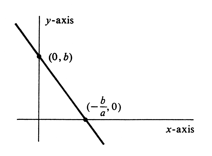
We shall commonly use lower-case letters at the beginning of the alphabet, e.g., [math]a[/math], [math]b[/math], [math]c[/math],..., to denote both constants and constant functions. Example \label{exam 1.3.4} Consider the function [math]ax + b[/math], where [math]a[/math] and [math]b[/math] are constants, [math]a \neq 0[/math], and [math]x[/math] is an independent variable. The graph of this function is a straight line that cuts the [math]y[/math]-axis at [math]b[/math] and the [math]x[/math]-axis at [math]-\frac{b}{a}[/math]. It is drawn in Figure.

This function is the sum of the constant function [math]b[/math] and the function which is the product of the constant function [math]a[/math] and the identity function [math]x[/math].

General references

Doyle, Peter G. (2008). "Crowell and Slesnick's Calculus with Analytic Geometry" (PDF). Retrieved Oct 29, 2024.