guide:956af30164

[math] \newcommand{\ex}[1]{\item } \newcommand{\sx}{\item} \newcommand{\x}{\sx} \newcommand{\sxlab}[1]{} \newcommand{\xlab}{\sxlab} \newcommand{\prov}[1] {\quad #1} \newcommand{\provx}[1] {\quad \mbox{#1}} \newcommand{\intext}[1]{\quad \mbox{#1} \quad} \newcommand{\R}{\mathrm{\bf R}} \newcommand{\Q}{\mathrm{\bf Q}} \newcommand{\Z}{\mathrm{\bf Z}} \newcommand{\C}{\mathrm{\bf C}} \newcommand{\dt}{\textbf} \newcommand{\goesto}{\rightarrow} \newcommand{\ddxof}[1]{\frac{d #1}{d x}} \newcommand{\ddx}{\frac{d}{dx}} \newcommand{\ddt}{\frac{d}{dt}} \newcommand{\dydx}{\ddxof y} \newcommand{\nxder}[3]{\frac{d^{#1}{#2}}{d{#3}^{#1}}} \newcommand{\deriv}[2]{\frac{d^{#1}{#2}}{dx^{#1}}} \newcommand{\dist}{\mathrm{distance}} \newcommand{\arccot}{\mathrm{arccot\:}} \newcommand{\arccsc}{\mathrm{arccsc\:}} \newcommand{\arcsec}{\mathrm{arcsec\:}} \newcommand{\arctanh}{\mathrm{arctanh\:}} \newcommand{\arcsinh}{\mathrm{arcsinh\:}} \newcommand{\arccosh}{\mathrm{arccosh\:}} \newcommand{\sech}{\mathrm{sech\:}} \newcommand{\csch}{\mathrm{csch\:}} \newcommand{\conj}[1]{\overline{#1}} \newcommand{\mathds}{\mathbb} [/math]

When we speak of the plane in this book, we assume, unless otherwise stated, that a pair of coordinate axes has been chosen. As a result, we identify the set of points in the plane with the set [math]R^2[/math] of all ordered pairs of real numbers. A convenient notation for a function [math]P[/math] whose domain is an interval [math]I[/math] of real numbers and whose range is a subset of the plane is [math]P : I \rightarrow R^2[/math]. Every function [math]P : I \rightarrow R^2[/math] defines two coordinate functions, the functions which assign to every [math]t[/math] in [math]I[/math] the two coordinates of the point [math]P(t)[/math]. If we denote the first coordinate function by [math]f[/math], and the second one by [math]g[/math], then they are defined by the equation

[[math]] \begin{equation} P(t) = (f(t), g(t)), \;\;\;\mbox{for every $t$ in $I$.} \label{eq10.1.1} \end{equation} [[/math]]

Conversely, of course, every ordered pair of real-valued functions [math]f[/math] and [math]g[/math] with an interval [math]I[/math] as common domain defines a function [math]P : I \rightarrow R^2[/math] by equation (1). Since the first and second coordinates of an element of [math]R^2[/math] are usually the [math]x[/math]- and [math]y[/math]-coordinates, respectively, we may alternatively define a function [math]P : I \rightarrow R^2[/math] by a pair of equations

[[math]] \left \{ \begin{array}{l} x = f(t), \\ y = g(t), \end{array} \right . [[/math]]

where [math]f[/math] and [math]g[/math] are real-valued functions with domain [math]I[/math]. Then, for every [math]t[/math] in [math]I[/math], we have [math]P(t) = (x, y) = (f(t), g(t))[/math]. It is also common practice to denote the coordinate functions themselves by [math]x[/math] and [math]y[/math]. When this is done, we do not hesitate to write the equations [math]x = x(t)[/math] and [math]y = y(t)[/math], and the function [math]P : I \rightarrow R^2[/math] is defined by

[[math]] P(t) = (x(t), y(t)), \;\;\;\mbox{for every $t$ in $I$.} [[/math]]

A function [math]P : I \rightarrow R^2[/math] is said to be continuous at [math]t_0[/math] if both coordinate functions are continuous at [math]t_0[/math]. If the coordinate functions are denoted by [math]x[/math] and [math]y[/math], then we define

[[math]] \lim_{t \rightarrow t_0} P(t) = (\lim_{t \rightarrow t_0} x(t), \lim_{t \rightarrow t_0} y(t)). [[/math]]

As a result, the definition of continuity for [math]P[/math] is entirely analogous to that for a real-valued function: [math]P[/math] is continuous at [math]t_0[/math] if [math]t_0[/math] is in the domain of [math]P[/math] and if [math]\lim_{t \rightarrow t_0} P(t) = P(t_0)[/math]. As before, the function [math]P[/math] is simply said to be continuous if it is continuous at every number in its domain. A curve in the plane is by definition a subset of [math]R^2[/math] which is the range of some continuous function [math]P : I \rightarrow R^2[/math]. Every curve is the range of many such functions, and, as a result, it is necessary to choose our terminology carefully. We shall call a continuous function [math]P : I \rightarrow R^2[/math], a parametrization of the curve [math]C[/math] which is the range of [math]P[/math], and we shall say that [math]C[/math] is parametrically defined by [math]P : I \rightarrow R^2[/math]. The points of the curve [math]C[/math] obviously consist of the set of all points [math]P(t)[/math], for every [math]t[/math] in [math]I[/math]. By a parametrized curve we shall mean the range of a specified continuous function [math]P : I \rightarrow R^2[/math]. Speaking more casually, we shall refer to the curve defined parametrically by

[[math]] P(t)= (x(t), y(t)), [[/math]]

or, equivalently, to the curve defined parametrically by the equations

[[math]] \left \{ \begin{array}{l} x = x(t), \\ y = y(t), \end{array} \right . [[/math]]

for every [math]t[/math] in some interval [math]I[/math] which is the common domain of the continuous functions [math]x[/math] and [math]y[/math]. If [math]t[/math] is regarded as an independent variable, it is called the parameter of the parametrized curve.

Example

Draw the curve defined parametrically by

[[math]] P(t) = (t^2, t), \;\;\; -\infty \lt t \lt \infty. [[/math]]

This is, of course, also the curve defined by the equations

[[math]] \left \{ \begin{array}{l} x = t^2,\\ y = t, \;\;\; -\infty \lt t \lt \infty. \end{array} \right . [[/math]]

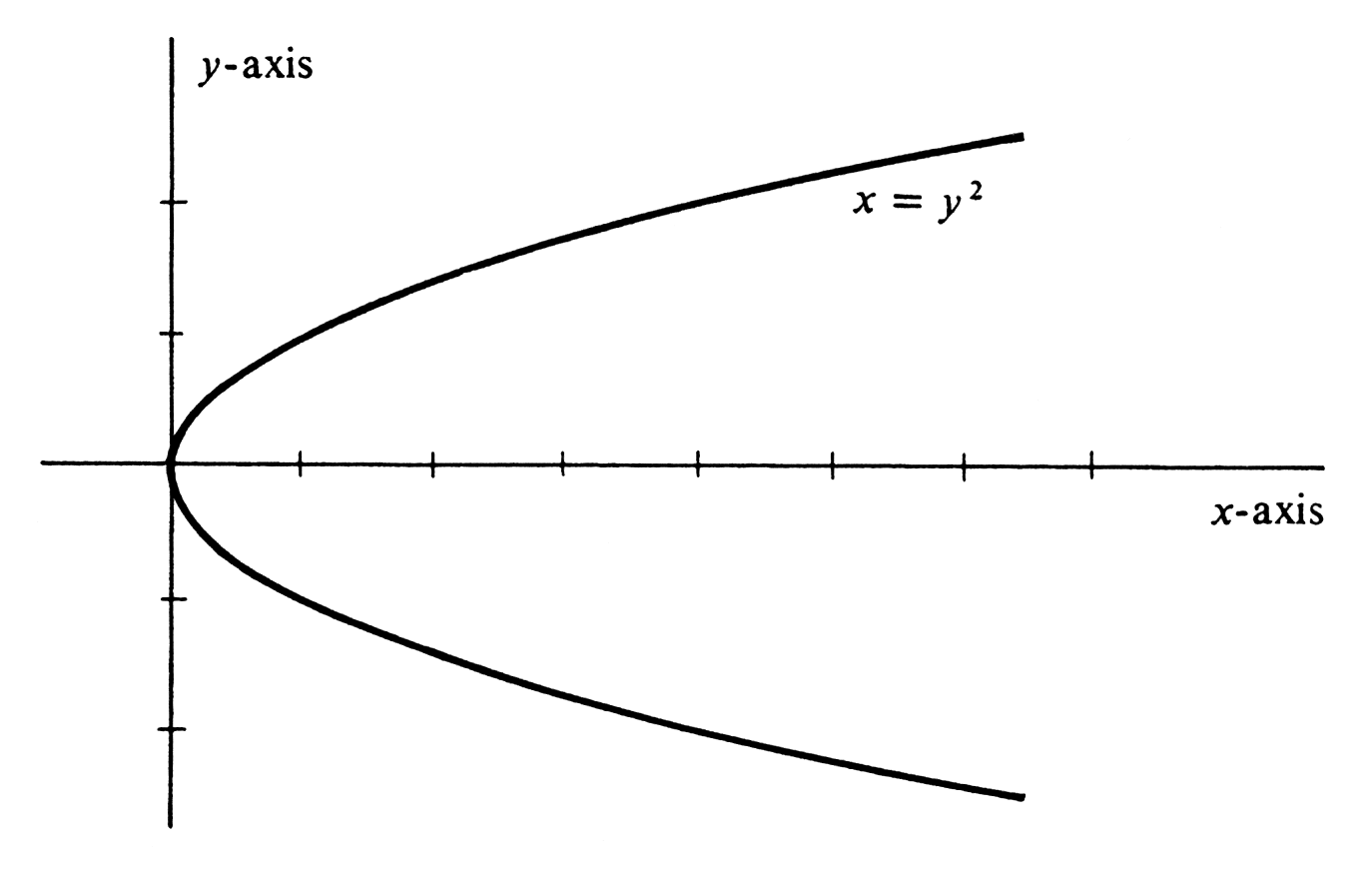
It is plotted in Figure 1. Since the set of all points [math](x, y)[/math] which satisfy the above two equations is equal to the set of all points [math](x, y)[/math] such that [math]x = y^2[/math], we recognize the curve as a parabola.

File:Guide c5467 scanfig10 1.png

t	(x, y)
0	(0, 0)
1	(1, 1)
2	(4, 2)

\medskip It is worth noting that every curve which we have previously encountered as the graph of a continuous function [math]f[/math] can be defined parametrically. The graph is the set of all points [math](x, y)[/math] such that [math]x[/math] is in the domain of [math]f[/math] and such that [math]y = f(x)[/math]. This set is obviously equal to the set of all points [math](x, y)[/math] such that

[[math]] \begin{equation} \left \{ \begin{array}{l} x = t,\\ y = f(t), \;\;\;\mbox{and $t$ is in the domain of $f$.} \end{array} \right . \label{eq10.1.2} \end{equation} [[/math]]

Hence the graph of [math]f[/math] is defined parametrically by equations (2). A function [math]P : I \rightarrow R^2[/math] is differentiable at [math]t_0[/math] if the derivatives of both coordinate functions exist at [math]t_0[/math]. Moreover, following the usual style, we say that [math]P[/math] is a differentiable function if it is differentiable at every number in its domain. This terminology is also applied to parametrized curves. That is, a curve defined parametrically by [math]P : I \rightarrow R^2[/math] is said to be differentiable at [math]t_0[/math], or simply differentiable, according as [math]P[/math] is differentiable at [math]t_0[/math], or is a differentiable function.

Example

Draw and identify the curve [math]C[/math] defined parametrically by

[[math]] P(t) = (x(t), y(t)) = (4\cos t, 3\sin t), [[/math]]

for every real number [math]t[/math]. If [math](x, y)[/math] is an arbitrary point on the curve, then

[[math]] \{ \begin{array}{l} x = 4 \cos t, \\ y = 3 \sin t, \end{array} [[/math]]

for some value of [math]t[/math]. Hence, [math]\frac{x}{4} = \cos t[/math] and [math]\frac{y}{3} = \sin t[/math], and, consequently,

[[math]] \frac{x^2}{16} + \frac{y^2}{9} = \cos^2 t + \sin^2 t = 1 . [[/math]]

Thus for every point [math](x, y)[/math] on the curve, we have shown that

[[math]] \begin{equation} \frac{x^2}{16} + \frac{y^2}{9} = 1. \label{eq10.1.3} \end{equation} [[/math]]

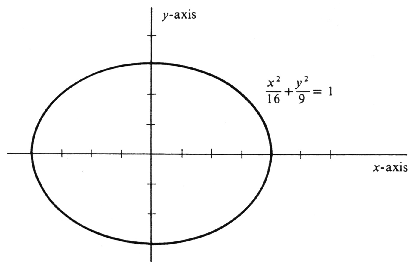
The latter is an equation of the ellipse shown in Figure 2, and it follows that the curve [math]C[/math] is a subset of the ellipse. Conversely, let [math](x, y)[/math] be an arbitrary point on the ellipse. Then [math]|x| \leq 4[/math], and so there exists a number [math]t[/math] such that [math]x = 4 \cos t[/math]. Since [math]\cos t = \cos(-t)[/math] and [math]\sin t = -\sin(-t)[/math], we may choose [math]t[/math] so that [math]\sin t[/math] and [math]y[/math] have the same sign. Then, solving equation (3) for [math]y[/math] and setting [math]x = 4 \cos t[/math], we obtain

File:Guide c5467 scanfig10 2.png

[[math]] \begin{eqnarray*} y^2 &=& 9 \Big(1 - \frac{x^2}{16} \Big) = 9 \Big(1 - \frac{16 \cos^2 t}{16} \Big) = 9(1 - \cos^2 t) \\ &=& 9 \sin^2t. \end{eqnarray*} [[/math]]

Since [math]y[/math] and [math]\sin t[/math] have the same sign, it follows that [math]y = 3 \sin t[/math]. We have therefore proved that, if [math](x, y)[/math] is an arbitrary point on the ellipse, then there exists a real number [math]t[/math] such that

[[math]] (x, y) = (4 \cos t, 3 \sin t) = P(t). [[/math]]

That is, every point on the ellipse also lies on [math]C[/math]. We have already shown that the converse is true, and we therefore conclude that the parametrized curve [math]C[/math] is equal to the ellipse.

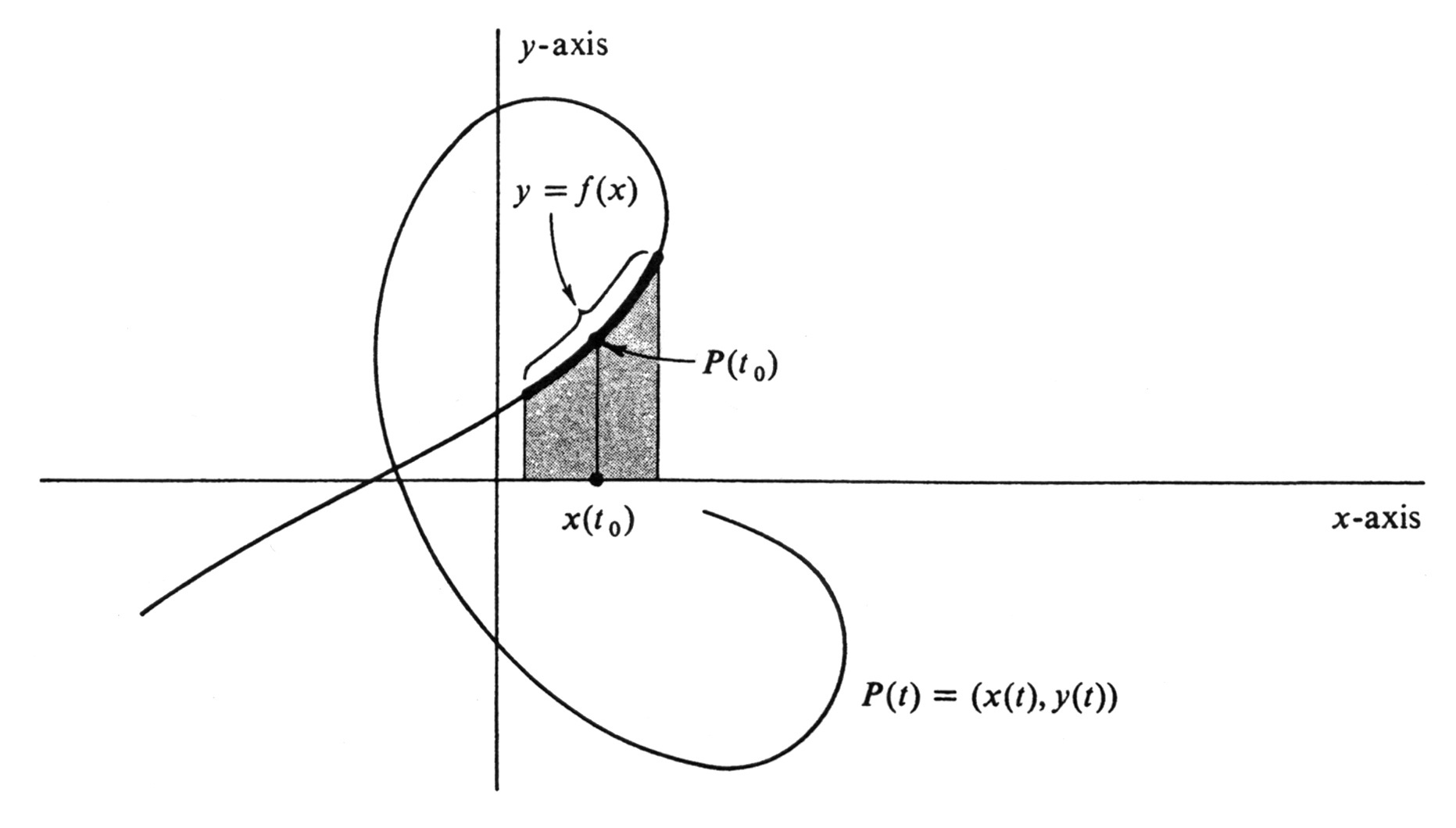
Consider a curve [math]C[/math] defined parametrically by a differentiable function [math]P : I \rightarrow R^2[/math], and let [math]t_0[/math] be an interior point of the interval [math]I[/math]. A typical example is shown in Figure 3. Generally it will not be the case that the whole curve is a function of [math]x[/math], since there may be distinct points on [math]C[/math] with the same [math]x[/math]-coordinate. However, it can happen that a subset of [math]C[/math] containing the point [math]P(t_0)[/math] is a differentiable function. Such a subset is shown in Figure 3, drawn with a heavy line. Thus if [math]P(t) = (x(t), y(t))[/math] for every [math]t[/math] in [math]I[/math], then there may exist a differentiable function [math]f[/math] such that

File:Guide c5467 scanfig10 3.png

[[math]] \begin{equation} y(t) = f(x(t)), \label{eq10.1.4} \end{equation} [[/math]]

for every [math]t[/math] in some subinterval of [math]I[/math] containing [math]t_0[/math] in its interior. If such a function does exist, we shall say that [math]y[/math] is a differentiable function of [math]x[/math] on the parametrized curve [math]P(t) = (x(t), y(t))[/math] in a neighborhood of the point [math]P(t_0)[/math]. Applying the Chain Rule to equation (4), we obtain

[[math]] y'(t) = f'(x(t)) x'(t) . [[/math]]

Hence

[[math]] \begin{equation} f'(x(t)) = \frac{y'(t)}{x'(t)}, \label{eq10.1.5} \end{equation} [[/math]]

for every [math]t[/math] in the subinterval, for which [math]x'(t) \neq 0[/math]. If we write [math]y = f(x)[/math] and use the differential notation for the derivative, formula (5) becomes

[[math]] \begin{equation} \frac{dy}{dx} = \frac{\frac{dy}{dt}}{\frac{dx}{dt}}. \label{eq10.1.6} \end{equation} [[/math]]

It should be apparent that [math]f'(x(t))[/math], or, equivalently, [math]\frac{dy}{dx}[/math] at [math]t[/math], is equal to the slope of the curve [math]C[/math] at the point [math]P(t)[/math].

Example

Find the slope, when [math]t = \frac{\pi}{3}[/math], of the parametrized ellipse in Example 2. The parametrization is defined by the equations

[[math]] \left \{ \begin{array}{l} x= 4\cos t, \\ y = 3 \sin t. \end{array} \right. [[/math]]

We shall assume the analytic result that [math]y[/math] is defined as a differentiable function of [math]x[/math] in a neighborhood of the point

[[math]] \Big(4 \cos \frac{\pi}{3}, 3 \sin \frac{\pi}{3} \Big). [[/math]]

Since

[[math]] \Big(4 \cos \frac{\pi}{3}, 3 \sin \frac{\pi}{3} \Big) = \Big(4 \cdot \frac{1}{2}, 3 \cdot \frac{\sqrt 3}{2} \Big) = \Big(2 , \frac{3 \sqrt 3}{2} \Big) , [[/math]]

one can see by simply looking at Figure 2 that this should certainly be true since the curve passes smoothly through the point and, in the immediate vicinity of the point, does not double back on itself. We have

[[math]] \begin{eqnarray*} \frac{dx}{dt} &=& \frac{d}{dt} 4 \cos t = - 4 \sin t ,\\ \frac{dy}{dt} &=& \frac{d}{dt} 3 \sin t = 3 \cos t , \end{eqnarray*} [[/math]]

and so

[[math]] \begin{eqnarray*} \frac{dx}{dt}\Big|_{t=\pi/3} &=& -4 \sin \frac{\pi}{3} = -4 \frac{\sqrt 3}{2} = - 2\sqrt 3, \\ \frac{dy}{dt}\Big|_{t=\pi/3} &=& 3 \cos \frac{\pi}{3} = \frac{3}{2} . \end{eqnarray*} [[/math]]

Hence, by formula (6), the slope is equal to

[[math]] \frac{dy}{dx}\Big|_{t=\pi/3} = \frac{\frac{dy}{dt}\Big|_{t=\pi/3}}{\frac{dx}{dt}\Big|_{t=\pi/3}} = \frac{\frac{3}{2}}{-2 \sqrt 3} = - \frac{3}{4 \sqrt 3} . [[/math]]

The problem of giving analytic conditions which imply that [math]y[/math] is a differentiable function of [math]x[/math] on a parametrized curve in the neighborhood of a point is akin to the problem of determining when an equation [math]F(x, y) = c[/math] implicitly defines [math]y[/math] as a differentiable function of [math]x[/math] in a neighborhood of a point. As mentioned on page 81, the latter is solved by the Implicit Function Theorem, and the techniques needed here are similar. As a final example, let us consider the curve traced by a point fixed on the circumference of a wheel as the wheel rolls along a straight line. We take the [math]x[/math]-axis for the straight line. The radius of the wheel we denote by [math]a[/math], and the point on the circumference by [math](x,y)[/math]. If we assume that the point passes through the origin as the wheel rolls by to the right, then the curve is defined parametrically by the equations

[[math]] \left \{ \begin{array}{l} x = a(\theta - \sin \theta),\\ y = a(1 - \cos \theta), \;\;\; -\infty \lt \theta \lt \infty, \end{array} \right . [[/math]]

where the parameter [math]\theta[/math] is the radian measure of the angle with vertex the center of the wheel, initial side the half-line pointing vertically downward, and terminal side the half-line through [math](x, y)[/math] (see Figure 4). (An alternative geometric interpretation of the parameter is that [math]a\theta[/math] is the coordinate of the point of tangency of the wheel on the [math]x[/math]-axis.) The curve is called a cycloid. Note that the parametric equations are quite simple, whereas it would be difficult to express [math]y[/math] as a function of [math]x[/math].

File:Guide c5467 scanfig10 4.png

General references

Doyle, Peter G. (2008). "Crowell and Slesnick's Calculus with Analytic Geometry" (PDF). Retrieved Oct 29, 2024.