guide:E0f9e256bf: Difference between revisions
No edit summary |
mNo edit summary |
||
| Line 1: | Line 1: | ||
==Mean Squared Error== | |||
In [[wikipedia:statistics|statistics]], the '''mean squared error''' ('''MSE''')<ref name=":1">{{Cite web|title=Mean Squared Error (MSE)|url=https://www.probabilitycourse.com/chapter9/9_1_5_mean_squared_error_MSE.php|access-date=2020-09-12|website=www.probabilitycourse.com}}</ref> or '''mean squared deviation''' ('''MSD''') of an [[wikipedia:estimator|estimator]] (of a procedure for estimating an unobserved quantity) measures the [[wikipedia:expected value|average]] of the squares of the [[wikipedia:Error (statistics)|errors]]—that is, the average squared difference between the estimated values and the actual value. MSE is a [[wikipedia:risk function|risk function]], corresponding to the [[wikipedia:expected value|expected value]] of the [[wikipedia:squared error loss|squared error loss]].<ref>{{cite book |title=Mathematical Statistics: Basic Ideas and Selected Topics |volume=I |edition=Second |last1=Bickel |first1=Peter J. |authorlink1=Peter J. Bickel |last2=Doksum |first2=Kjell A. |year=2015 |page=20 |quotation="If we use quadratic loss, our risk function is called the ''mean squared error'' (MSE) ..."}}</ref> The fact that MSE is almost always strictly positive (and not zero) is because of [[wikipedia:randomness|randomness]] or because the estimator [[wikipedia:Omitted-variable bias|does not account for information]] that could produce a more accurate estimate.<ref name="pointEstimation">{{cite book |first1=E. L. |last1=Lehmann |first2=George |last2=Casella |title=Theory of Point Estimation |publisher=Springer |location=New York |year=1998 |edition=2nd |isbn=978-0-387-98502-2 |mr=1639875}}</ref> In [[wikipedia:machine learning|machine learning]], specifically [[wikipedia:empirical risk minimization|empirical risk minimization]], MSE may refer to the ''empirical'' risk (the average loss on an observed data set), as an estimate of the true MSE (the true risk: the average loss on the actual population distribution). | |||
The MSE is a measure of the quality of an estimator. As it is derived from the square of [[wikipedia:Euclidean distance|Euclidean distance]], it is always a positive value that decreases as the error approaches zero. | |||
The MSE is the second [[wikipedia:moment (mathematics)|moment]] (about the origin) of the error, and thus incorporates both the [[wikipedia:variance|variance]] of the estimator (how widely spread the estimates are from one [[wikipedia:data sample|data sample]] to another) and its [[wikipedia:Bias of an estimator|bias]] (how far off the average estimated value is from the true value). For an [[wikipedia:unbiased estimator|unbiased estimator]], the MSE is the variance of the estimator. Like the variance, MSE has the same units of measurement as the square of the quantity being estimated. In an analogy to [[wikipedia:standard deviation|standard deviation]], taking the square root of MSE yields the ''root-mean-square error'' or ''[[wikipedia:root-mean-square deviation|root-mean-square deviation]]'' (RMSE or RMSD), which has the same units as the quantity being estimated; for an unbiased estimator, the RMSE is the square root of the [[wikipedia:variance|variance]], known as the [[wikipedia:standard error|standard error]]. | |||
==Definition and basic properties== | |||
The MSE either assesses the quality of a ''[[wikipedia:predictor (statistics)|predictor]]'' (i.e., a function mapping arbitrary inputs to a sample of values of some [[wikipedia:random variable|random variable]]), or of an ''[[wikipedia:estimator|estimator]]'' (i.e., a [[wikipedia:mathematical function|mathematical function]] mapping a [[wikipedia:Sample (statistics)|sample]] of data to an estimate of a [[wikipedia:Statistical parameter|parameter]] of the [[wikipedia:Statistical population|population]] from which the data is sampled). The definition of an MSE differs according to whether one is describing a predictor or an estimator. | |||
===Predictor=== | |||
If a vector of <math>n</math> predictions is generated from a sample of <math>n</math> data points on all variables, and <math>Y</math> is the vector of observed values of the variable being predicted, with <math>\hat{Y}</math> being the predicted values (e.g. as from a [[wikipedia:least-squares fit|least-squares fit]]), then the within-sample MSE of the predictor is computed as | |||
<math display="block">\operatorname{MSE}=\frac{1}{n} \sum_{i=1}^n \left(Y_i-\hat{Y_i}\right)^2.</math> | |||
In other words, the MSE is the ''mean'' <math display="inline">\left(\frac{1}{n} \sum_{i=1}^n \right)</math> of the ''squares of the errors'' <math display="inline">\left(Y_i-\hat{Y_i}\right)^2</math>. This is an easily computable quantity for a particular sample (and hence is sample-dependent). | |||
In [[wikipedia:Matrix_multiplication|matrix]] notation, | |||
<math display="block">\operatorname{MSE}=\frac{1}{n}\sum_{i=1}^n(e_i)^2=\frac{1}{n}\mathbf e^\mathsf T \mathbf e</math> | |||
where <math>e_i</math> is <math> (Y_i-\hat{Y_i}) </math> and <math>\mathbf e</math> is the <math> n \times 1 </math> column vector. | |||
The MSE can also be computed on ''q ''data points that were not used in estimating the model, either because they were held back for this purpose, or because these data have been newly obtained. Within this process, known as [[wikipedia:Statistical learning theory|statistical learning]], the MSE is often called the [[wikipedia:test MSE|test MSE]],<ref>{{cite book | |||
|first1=James | |||
|last1=Gareth | |||
|first2=Daniela | |||
|last2=Witten | |||
|first3=Trevor | |||
|last3=Hastie | |||
|first4=Rob | |||
|last4=Tibshirani | |||
|date=2021 | |||
|title=An Introduction to Statistical Learning: with Applications in R | |||
|url=https://www.statlearning.com/ | |||
|publisher=Springer | |||
|isbn=978-1071614174 | |||
}}</ref> and is computed as | |||
<math display="block">\operatorname{MSE} = \frac{1}{q} \sum_{i=n+1}^{n+q} \left(Y_i-\hat{Y_i}\right)^2.</math> | |||
===Estimator=== | |||
The MSE of an estimator <math>\hat{\theta}</math> with respect to an unknown parameter <math>\theta</math> is defined as<ref name=":1" /> | |||
<math display="block">\operatorname{MSE}(\hat{\theta})=\operatorname{E}_{\theta}\left[(\hat{\theta}-\theta)^2\right].</math> | |||
This definition depends on the unknown parameter, but the MSE is ''a priori'' a property of an estimator. The MSE could be a function of unknown parameters, in which case any ''estimator'' of the MSE based on estimates of these parameters would be a function of the data (and thus a random variable). If the estimator <math>\hat{\theta}</math> is derived as a sample statistic and is used to estimate some population parameter, then the expectation is with respect to the sampling distribution of the sample statistic. | |||
The MSE can be written as the sum of the [[wikipedia:variance|variance]] of the estimator and the squared [[wikipedia:Bias_of_an_estimator|bias]] of the estimator, providing a useful way to calculate the MSE and implying that in the case of unbiased estimators, the MSE and variance are equivalent.<ref name="wackerly">{{cite book |first1=Dennis |last1=Wackerly |first2=William|last2=Mendenhall |first3=Richard L.|last3=Scheaffer |title=Mathematical Statistics with Applications |publisher=Thomson Higher Education|location=Belmont, CA, USA |year=2008 |edition=7 |isbn=978-0-495-38508-0}}</ref> | |||
<math display="block">\operatorname{MSE}(\hat{\theta})=\operatorname{Var}_{\theta}(\hat{\theta})+ \operatorname{Bias}(\hat{\theta},\theta)^2.</math> | |||
But in real modeling case, MSE could be described as the addition of model variance, model bias, and irreducible uncertainty (see [[wikipedia:Bias–variance tradeoff|Bias–variance tradeoff]]). According to the relationship, the MSE of the estimators could be simply used for the [[wikipedia:Efficiency (statistics)|efficiency]] comparison, which includes the information of estimator variance and bias. This is called MSE criterion. | |||
===Examples=== | |||
====Mean==== | |||
Suppose we have a random sample of size <math>n</math> from a population, <math>X_1,\dots,X_n</math>. Suppose the sample units were chosen [[wikipedia:Sampling with replacement|with replacement]]. That is, the <math>n</math> units are selected one at a time, and previously selected units are still eligible for selection for all <math>n</math> draws. The usual estimator for the <math>\mu</math> is the sample average | |||
<math display="block">\overline{X}=\frac{1}{n}\sum_{i=1}^n X_i </math> | |||
which has an expected value equal to the true mean <math>\mu</math> (so it is unbiased) and a mean squared error of | |||
<math display="block">\operatorname{MSE}\left(\overline{X}\right)=\operatorname{E}\left[\left(\overline{X}-\mu\right)^2\right]=\left(\frac{\sigma}{\sqrt{n}}\right)^2= \frac{\sigma^2}{n}</math> | |||
where <math>\sigma^2</math> is the [[wikipedia:Sample variance#Population variance|population variance]]. | |||
For a [[wikipedia:Gaussian distribution|Gaussian distribution]], this is the [[wikipedia:best unbiased estimator|best unbiased estimator]] (i.e., one with the lowest MSE among all unbiased estimators), but not, say, for a [[wikipedia:Uniform distribution (continuous)|uniform distribution]]. | |||
====Variance==== | |||
The usual estimator for the variance is the ''corrected [[wikipedia:sample variance|sample variance]]:'' | |||
<math display="block">S^2_{n-1} = \frac{1}{n-1}\sum_{i=1}^n\left(X_i-\overline{X} \right)^2 =\frac{1}{n-1}\left(\sum_{i=1}^n X_i^2-n\overline{X}^2\right).</math> | |||
This is unbiased (its expected value is <math>\sigma^2</math>), hence also called the ''unbiased sample variance,'' and its MSE is<ref>{{cite book | last = Mood |first=A. | last2 = Graybill |first2=F. |last3=Boes |first3=D. | title = Introduction to the Theory of Statistics | url = https://archive.org/details/introductiontoth00mood_706 | url-access = limited |page=[https://archive.org/details/introductiontoth00mood_706/page/n241 229] | edition = 3rd | publisher = McGraw-Hill | year = 1974}}</ref> | |||
<math display="block">\operatorname{MSE}(S^2_{n-1})= \frac{1}{n} \left(\mu_4-\frac{n-3}{n-1}\sigma^4\right) =\frac{1}{n} \left(\gamma_2+\frac{2n}{n-1}\right)\sigma^4,</math> | |||
where <math>\mu_4</math> is the fourth [[wikipedia:central moment|central moment]] of the distribution or population, and <math>\gamma_2=\mu_4/\sigma^4-3</math> is the [[wikipedia:excess kurtosis|excess kurtosis]]. | |||
However, one can use other estimators for <math>\sigma^2</math> which are proportional to <math>S^2_{n-1}</math>, and an appropriate choice can always give a lower mean squared error. If we define | |||
<math display="block">S^2_a = \frac{n-1}{a}S^2_{n-1}= \frac{1}{a}\sum_{i=1}^n\left(X_i-\overline{X}\,\right)^2</math> | |||
then we calculate: | |||
<math display="block">\begin{align*} | |||
\operatorname{MSE}(S^2_a) | |||
&=\operatorname{E}\left[\left(\frac{n-1}{a} S^2_{n-1}-\sigma^2\right)^2 \right] \\ | |||
&= \operatorname{E}\left[ \frac{(n-1)^2}{a^2} S^4_{n-1} -2 \left ( \frac{n-1}{a} S^2_{n-1} \right ) \sigma^2 + \sigma^4 \right ] \\ | |||
&= \frac{(n-1)^2}{a^2} \operatorname{E}\left[ S^4_{n-1} \right ] - 2 \left ( \frac{n-1}{a}\right ) \operatorname{E}\left[ S^2_{n-1} \right ] \sigma^2 + \sigma^4 \\ | |||
&= \frac{(n-1)^2}{a^2} \operatorname{E}\left[ S^4_{n-1} \right ] - 2 \left ( \frac{n-1}{a}\right ) \sigma^4 + \sigma^4 && \operatorname{E}\left[ S^2_{n-1} \right ] = \sigma^2 \\ | |||
&= \frac{(n-1)^2}{a^2} \left ( \frac{\gamma_2}{n} + \frac{n+1}{n-1} \right ) \sigma^4- 2 \left ( \frac{n-1}{a}\right ) \sigma^4+\sigma^4 && \operatorname{E}\left[ S^4_{n-1} \right ] = \operatorname{MSE}(S^2_{n-1}) + \sigma^4 \\ | |||
&=\frac{n-1}{n a^2} \left ((n-1)\gamma_2+n^2+n \right ) \sigma^4- 2 \left ( \frac{n-1}{a}\right ) \sigma^4+\sigma^4 | |||
\end{align*}</math> | |||
This is minimized when | |||
<math display="block">a=\frac{(n-1)\gamma_2+n^2+n}{n} = n+1+\frac{n-1}{n}\gamma_2.</math> | |||
For a [[wikipedia:Gaussian distribution|Gaussian distribution]], where <math>\gamma_2=0</math>, this means that the MSE is minimized when dividing the sum by <math>a=n+1</math>. The minimum excess kurtosis is <math>\gamma_2=-2</math>,{{efn|1=This can be proved by [[wikipedia:Jensen's inequality|Jensen's inequality]] as follows. The fourth [[wikipedia:central moment|central moment]] is an upper bound for the square of variance, so that the least value for their ratio is one, therefore, the least value for the [[wikipedia:excess kurtosis|excess kurtosis]] is −2, achieved, for instance, by a Bernoulli with ''p''=1/2.}} which is achieved by a [[wikipedia:Bernoulli distribution|Bernoulli distribution]] with ''p'' = 1/2 (a coin flip), and the MSE is minimized for <math>a=n-1+\tfrac{2}{n}.</math> Hence regardless of the kurtosis, we get a "better" estimate (in the sense of having a lower MSE) by scaling down the unbiased estimator a little bit; this is a simple example of a [[wikipedia:shrinkage estimator|shrinkage estimator]]: one "shrinks" the estimator towards zero (scales down the unbiased estimator). | |||
Further, while the corrected sample variance is the [[wikipedia:best unbiased estimator|best unbiased estimator]] (minimum mean squared error among unbiased estimators) of variance for Gaussian distributions, if the distribution is not Gaussian, then even among unbiased estimators, the best unbiased estimator of the variance may not be <math>S^2_{n-1}.</math> | |||
====Gaussian distribution==== | |||
The following table gives several estimators of the true parameters of the population, μ and σ<sup>2</sup>, for the Gaussian case.<ref>{{cite book | last = DeGroot | first = Morris H. | author-link = wikipedia:Morris H. DeGroot | title = Probability and Statistics | edition = 2nd | publisher = Addison-Wesley | year = 1980 | ref = degroot }}</ref> | |||
{| class="table table-bordered" | |||
! True value !! Estimator !! Mean squared error | |||
|- | |||
| <math>\theta=\mu</math> || <math>\hat{\theta}</math> = the unbiased estimator of the [[wikipedia:population mean|population mean]], <math>\overline{X}=\frac{1}{n}\sum_{i=1}^n(X_i)</math> || <math>\operatorname{MSE}(\overline{X})=\operatorname{E}((\overline{X}-\mu)^2)=\left(\frac{\sigma}{\sqrt{n}}\right)^2</math> | |||
|- | |||
| <math>\theta=\sigma^2</math> || <math>\hat{\theta}</math> = the unbiased estimator of the [[wikipedia:population variance|population variance]], <math>S^2_{n-1} = \frac{1}{n-1}\sum_{i=1}^n\left(X_i-\overline{X}\,\right)^2</math> || <math>\operatorname{MSE}(S^2_{n-1})=\operatorname{E}((S^2_{n-1}-\sigma^2)^2)=\frac{2}{n - 1}\sigma^4</math> | |||
|- | |||
| <math>\theta=\sigma^2</math> || <math>\hat{\theta}</math> = the biased estimator of the [[wikipedia:population variance|population variance]], <math>S^2_{n} = \frac{1}{n}\sum_{i=1}^n\left(X_i-\overline{X}\,\right)^2</math> || <math>\operatorname{MSE}(S^2_{n})=\operatorname{E}((S^2_{n}-\sigma^2)^2)=\frac{2n - 1}{n^2}\sigma^4</math> | |||
|- | |||
| <math>\theta=\sigma^2</math> || <math>\hat{\theta}</math> = the biased estimator of the [[wikipedia:population variance|population variance]], <math>S^2_{n+1} = \frac{1}{n+1}\sum_{i=1}^n\left(X_i-\overline{X}\,\right)^2</math> || <math>\operatorname{MSE}(S^2_{n+1})=\operatorname{E}((S^2_{n+1}-\sigma^2)^2)=\frac{2}{n + 1}\sigma^4</math> | |||
|} | |||
===Interpretation=== | |||
An MSE of zero, meaning that the estimator <math>\hat{\theta}</math> predicts observations of the parameter <math>\theta</math> with perfect accuracy, is ideal (but typically not possible). | |||
Values of MSE may be used for comparative purposes. Two or more [[wikipedia:statistical model|statistical model]]s may be compared using their MSEs—as a measure of how well they explain a given set of observations: An unbiased estimator (estimated from a statistical model) with the smallest variance among all unbiased estimators is the ''best unbiased estimator'' or MVUE ([[wikipedia:Minimum-variance unbiased estimator|Minimum-Variance Unbiased Estimator]]). | |||
Both [[wikipedia:analysis of variance|analysis of variance]] and [[wikipedia:linear regression|linear regression]] techniques estimate the MSE as part of the analysis and use the estimated MSE to determine the [[wikipedia:statistical significance|statistical significance]] of the factors or predictors under study. The goal of [[wikipedia:experimental design|experimental design]] is to construct experiments in such a way that when the observations are analyzed, the MSE is close to zero relative to the magnitude of at least one of the estimated treatment effects. | |||
In [[wikipedia:one-way analysis of variance|one-way analysis of variance]], MSE can be calculated by the division of the sum of squared errors and the degree of freedom. Also, the f-value is the ratio of the mean squared treatment and the MSE. | |||
===Loss function=== | |||
Squared error loss is one of the most widely used [[wikipedia:loss function|loss function]]s in statistics, though its widespread use stems more from mathematical convenience than considerations of actual loss in applications. [[wikipedia:Carl Friedrich Gauss|Carl Friedrich Gauss]], who introduced the use of mean squared error, was aware of its arbitrariness and was in agreement with objections to it on these grounds.<ref name="pointEstimation" /> The mathematical benefits of mean squared error are particularly evident in its use at analyzing the performance of [[wikipedia:linear regression|linear regression]], as it allows one to partition the variation in a dataset into variation explained by the model and variation explained by randomness. | |||
===Criticism=== | |||
The use of mean squared error without question has been criticized by the [[wikipedia:decision theory|decision theorist]] [[wikipedia:James Berger (statistician)|James Berger]]. Mean squared error is the negative of the expected value of one specific [[wikipedia:utility function|utility function]], the quadratic utility function, which may not be the appropriate utility function to use under a given set of circumstances. There are, however, some scenarios where mean squared error can serve as a good approximation to a loss function occurring naturally in an application.<ref>{{cite book | |||
|title=Statistical Decision Theory and Bayesian Analysis | |||
|url=https://archive.org/details/statisticaldecis00berg | |||
|url-access=limited | |||
|first=James O. |last=Berger |author-link=wikipedia:James Berger (statistician) | |||
|year=1985 | |||
|edition=2nd | |||
|publisher=Springer-Verlag |location=New York | |||
|isbn=978-0-387-96098-2 |mr=0804611 | |||
|chapter=2.4.2 Certain Standard Loss Functions |page=[https://archive.org/details/statisticaldecis00berg/page/n72 60] | |||
}}</ref> | |||
Like [[wikipedia:variance|variance]], mean squared error has the disadvantage of heavily weighting [[wikipedia:outliers|outliers]].<ref>{{cite journal | last1 = Bermejo | first1 = Sergio | last2 = Cabestany | first2 = Joan | year = 2001 | title = Oriented principal component analysis for large margin classifiers | journal = Neural Networks | volume = 14 | issue = 10| pages = 1447–1461 | doi=10.1016/S0893-6080(01)00106-X| pmid = 11771723 }}</ref> This is a result of the squaring of each term, which effectively weights large errors more heavily than small ones. This property, undesirable in many applications, has led researchers to use alternatives such as the [[wikipedia:mean absolute error|mean absolute error]], or those based on the [[wikipedia:median|median]]. | |||
In [[wikipedia:statistics|statistics]] and [[wikipedia:machine learning|machine learning]], the '''bias–variance tradeoff''' is the property of a model that the [[wikipedia:variance|variance]] of the parameter estimated across [[wikipedia:sample (statistics)|samples]] can be reduced by increasing the [[wikipedia:Bias_of_an_estimator|bias]] in the [[wikipedia:estimation theory|estimated]] [[wikipedia:statistical parameter|parameters]]. | |||
The '''bias–variance dilemma''' or '''bias–variance problem''' is the conflict in trying to simultaneously minimize these two sources of [[wikipedia:Errors and residuals in statistics|error]] that prevent [[wikipedia:supervised learning|supervised learning]] algorithms from generalizing beyond their [[wikipedia:training set|training set]]:<ref>{{cite journal |last1=Kohavi |first1=Ron |last2=Wolpert |first2=David H. |title=Bias Plus Variance Decomposition for Zero-One Loss Functions |journal=ICML |date=1996 |volume=96}}</ref><ref>{{cite journal |last1=Luxburg |first1=Ulrike V. |last2=Schölkopf |first2=B. |title=Statistical learning theory: Models, concepts, and results |journal=Handbook of the History of Logic |date=2011 |volume=10| page=Section 2.4}}</ref> | |||
* The [[wikipedia:Bias of an estimator|''bias'']] error is an error from erroneous assumptions in the learning [[wikipedia:algorithm|algorithm]]. High bias can cause an algorithm to miss the relevant relations between features and target outputs (underfitting). | |||
* The ''[[wikipedia:variance|variance]]'' is an error from sensitivity to small fluctuations in the training set. High variance may result from an algorithm modeling the random [[wikipedia:Noise (signal processing)|noise]] in the training data ([[wikipedia:overfitting|overfitting]]). | |||
The '''bias–variance decomposition''' is a way of analyzing a learning algorithm's [[wikipedia:expected value|expected]] [[wikipedia:generalization error|generalization error]] with respect to a particular problem as a sum of three terms, the bias, variance, and a quantity called the ''irreducible error'', resulting from noise in the problem itself. | |||
==Motivation== | |||
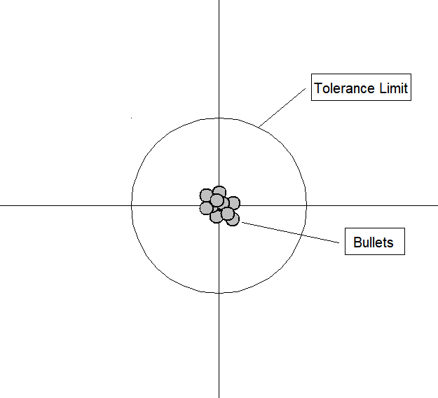
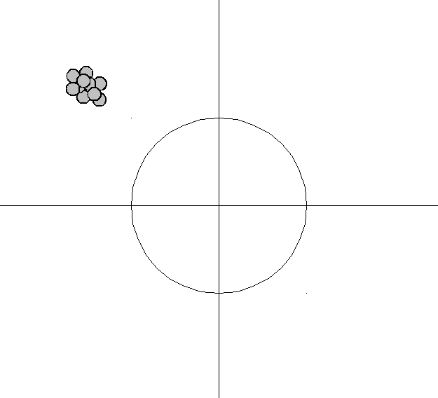
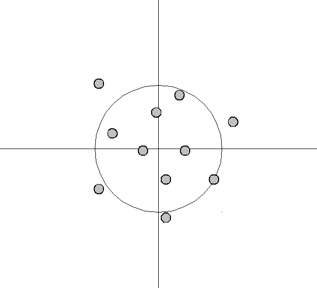
<gallery> | |||
File:En low bias low variance.png|bias low,variance low | |||
File:Truen bad prec ok.png|bias high,<br />variance low | |||
File:Truen ok prec bad.png|bias low,<br />variance high | |||
File:Truen bad prec bad.png|bias high,<br />variance high | |||
</gallery> | |||
The bias–variance tradeoff is a central problem in supervised learning. Ideally, one wants to [[wikipedia:Model selection|choose a model]] that both accurately captures the regularities in its training data, but also [[wikipedia:Generalization|generalizes]] well to unseen data. Unfortunately, it is typically impossible to do both simultaneously. High-variance learning methods may be able to represent their training set well but are at risk of overfitting to noisy or unrepresentative training data. In contrast, algorithms with high bias typically produce simpler models that may fail to capture important regularities (i.e. underfit) in the data. | |||
It is an often made [[wikipedia:Affirming the consequent|fallacy]]<ref name="nealThesis2019">{{cite arXiv |last=Neal |first=Brady |eprint=1912.08286 |title=On the Bias-Variance Tradeoff: Textbooks Need an Update |class=cs.LG |date=2019}}</ref><ref name="neal2018">{{cite arXiv |first1=Brady |last1=Neal |first2=Sarthak |last2=Mittal |first3=Aristide |last3=Baratin |first4=Vinayak |last4=Tantia |first5=Matthew |last5=Scicluna |first6=Simon |last6=Lacoste-Julien |first7=Ioannis |last7=Mitliagkas |eprint=1810.08591 |title=A Modern Take on the Bias-Variance Tradeoff in Neural Networks |class=cs.LG |date=2018}}</ref> to assume that complex models must have high variance; High variance models are 'complex' in some sense, but the reverse needs not be true. | |||
In addition, one has to be careful how to define complexity: In particular, the number of parameters used to describe the model is a poor measure of complexity. This is illustrated by an example adapted from:<ref>{{cite book |last1=Vapnik |first1=Vladimir |title=The nature of statistical learning theory |date=2000 |publisher=Springer-Verlag |location=New York |isbn=978-1-4757-3264-1 |url=https://dx.doi.org/10.1007/978-1-4757-3264-1}}</ref> The model <math>f_{a,b}(x)=a\sin(bx)</math> has only two parameters (<math>a,b</math>) but it can interpolate any number of points by oscillating with a high enough frequency, resulting in both a high bias and high variance. | |||
An analogy can be made to the relationship between [[wikipedia:Accuracy and precision|accuracy and precision]]. Accuracy is a description of bias and can intuitively be improved by selecting from only [[wikipedia:Sample space|local]] information. Consequently, a sample will appear accurate (i.e. have low bias) under the aforementioned selection conditions, but may result in underfitting. In other words, [[wikipedia:Training, validation, and test data sets|test data]] may not agree as closely with training data, which would indicate imprecision and therefore inflated variance. A graphical example would be a straight line fit to data exhibiting quadratic behavior overall. Precision is a description of variance and generally can only be improved by selecting information from a comparatively larger space. The option to select many data points over a broad sample space is the ideal condition for any analysis. However, intrinsic constraints (whether physical, theoretical, computational, etc.) will always play a limiting role. The limiting case where only a finite number of data points are selected over a broad sample space may result in improved precision and lower variance overall, but may also result in an overreliance on the training data (overfitting). This means that test data would also not agree as closely with the training data, but in this case the reason is due to inaccuracy or high bias. To borrow from the previous example, the graphical representation would appear as a high-order polynomial fit to the same data exhibiting quadratic behavior. Note that error in each case is measured the same way, but the reason ascribed to the error is different depending on the balance between bias and variance. To mitigate how much information is used from neighboring observations, a model can be [[wikipedia:smoothing|smoothed]] via explicit [[wikipedia:Regularization (mathematics)|regularization]], such as [[wikipedia:shrinkage (statistics)|shrinkage]]. | |||
==Bias–variance decomposition of mean squared error== | |||
Suppose that we have a training set consisting of a set of points <math>x_1, \dots, x_n</math> and real values <math>y_i</math> associated with each point <math>x_i</math>. We assume that there is a function with noise <math>y = f(x) + \varepsilon</math>, where the noise, <math>\varepsilon</math>, has zero mean and variance <math>\sigma^2</math>. | |||
We want to find a function <math>\hat{f}(x;D)</math>, that approximates the true function <math>f(x)</math> as well as possible, by means of some learning algorithm based on a training dataset (sample) <math>D=\{(x_1,y_1) \dots, (x_n, y_n)\}</math>. We make "as well as possible" precise by measuring the [[wikipedia:mean squared error|mean squared error]] between <math>y</math> and <math>\hat{f}(x;D)</math>: we want <math>(y - \hat{f}(x;D))^2</math> to be minimal, both for <math>x_1, \dots, x_n</math> ''and for points outside of our sample''. Of course, we cannot hope to do so perfectly, since the <math>y_i</math> contain noise <math>\varepsilon</math>; this means we must be prepared to accept an ''irreducible error'' in any function we come up with. | |||
Finding an <math>\hat{f}</math> that generalizes to points outside of the training set can be done with any of the countless algorithms used for supervised learning. It turns out that whichever function <math>\hat{f}</math> we select, we can decompose its [[wikipedia:expected value|expected]] error on an unseen sample <math>x</math> as follows:<ref name="islr">{{cite book |first1=Gareth |last1=James |first2=Daniela |last2=Witten |author-link2=wikipedia:Daniela Witten |first3=Trevor |last3=Hastie |author-link3=wikipedia:Trevor Hastie |first4=Robert |last4=Tibshirani |author-link4=wikipedia:Robert Tibshirani |title=An Introduction to Statistical Learning |publisher=Springer |year=2013 |url=http://www-bcf.usc.edu/~gareth/ISL/ }}</ref>{{rp|34}}<ref name="ESL">{{cite book |first1=Trevor |last1=Hastie |first2=Robert |last2=Tibshirani |first3=Jerome H. |last3=Friedman |author-link3=wikipedia:Jerome H. Friedman |year=2009 |title=The Elements of Statistical Learning |url=http://statweb.stanford.edu/~tibs/ElemStatLearn/ |access-date=2014-08-20 |archive-url=https://web.archive.org/web/20150126123924/http://statweb.stanford.edu/~tibs/ElemStatLearn/ |archive-date=2015-01-26 |url-status=dead }}</ref>{{rp|223}} | |||
<math display="block"> | |||
\operatorname{E}_{D, \varepsilon} \Big[\big(y - \hat{f}(x;D)\big)^2\Big] | |||
= \Big(\operatorname{Bias}_D\big[\hat{f}(x;D)\big] \Big) ^2 + \operatorname{Var}_D\big[\hat{f}(x;D)\big] + \sigma^2 | |||
</math> | |||
where | |||
<math display="block"> | |||
\operatorname{Bias}_D\big[\hat{f}(x;D)\big] = \operatorname{E}_D\big[\hat{f}(x;D)\big] - f(x) | |||
</math> | |||
and | |||
<math display="block"> | |||
\operatorname{Var}_D\big[\hat{f}(x;D)\big] = \operatorname{E}_D[\big(\operatorname{E}_D[\hat{f}(x;D)] - \hat{f}(x;D)\big)^2]. | |||
</math> | |||
The expectation ranges over different choices of the training set <math>D=\{(x_1,y_1) \dots, (x_n, y_n)\}</math>, all sampled from the same joint distribution <math>P(x,y)</math> which can for example be done via [[wikipedia:Bootstrapping (statistics)|bootstrapping]]. | |||
The three terms represent: | |||
* the square of the ''bias'' of the learning method, which can be thought of as the error caused by the simplifying assumptions built into the method. E.g., when approximating a non-linear function <math>f(x)</math> using a learning method for [[wikipedia:linear model|linear model]]s, there will be error in the estimates <math>\hat{f}(x)</math> due to this assumption; | |||
* the ''variance'' of the learning method, or, intuitively, how much the learning method <math>\hat{f}(x)</math> will move around its mean; | |||
* the irreducible error <math>\sigma^2</math>. | |||
Since all three terms are non-negative, the irreducible error forms a lower bound on the expected error on unseen samples.<ref name="islr" />{{rp|34}} | |||
The more complex the model <math>\hat{f}(x)</math> is, the more data points it will capture, and the lower the bias will be. However, complexity will make the model "move" more to capture the data points, and hence its variance will be larger. | |||
==Approaches== | |||
[[wikipedia:Dimensionality reduction|Dimensionality reduction]] and [[wikipedia:feature selection|feature selection]] can decrease variance by simplifying models. Similarly, a larger training set tends to decrease variance. Adding features (predictors) tends to decrease bias, at the expense of introducing additional variance. Learning algorithms typically have some tunable parameters that control bias and variance; for example, | |||
* [[wikipedia:linear model|linear]] and [[wikipedia:Generalized linear model|Generalized linear]] models can be [[wikipedia:Regularization (mathematics)|regularized]] to decrease their variance at the cost of increasing their bias.<ref>{{cite book |last=Belsley |first=David |title=Conditioning diagnostics : collinearity and weak data in regression |publisher=Wiley |location=New York (NY) |year=1991 |isbn=978-0471528890 }}</ref> | |||
* In [[wikipedia:artificial neural network|artificial neural network]]s, the variance increases and the bias decreases as the number of hidden units increase,<ref name="geman">{{cite journal |last1=Geman |first1=Stuart |author-link1=wikipedia:Stuart Geman |first2=Élie |last2=Bienenstock |first3=René |last3=Doursat |year=1992 |title=Neural networks and the bias/variance dilemma |journal=Neural Computation |volume=4 |pages=1–58 |doi=10.1162/neco.1992.4.1.1 |url=http://web.mit.edu/6.435/www/Geman92.pdf }}</ref> although this classical assumption has been the subject of recent debate.<ref name="neal2018" /> Like in GLMs, regularization is typically applied. | |||
* In [[wikipedia:k-nearest neighbor|''k''-nearest neighbor]] models, a high value of {{mvar|k}} leads to high bias and low variance (see below). | |||
* In [[wikipedia:instance-based learning|instance-based learning]], regularization can be achieved varying the mixture of [[wikipedia:prototype|prototype]]s and exemplars.<ref>{{cite journal |last1=Gagliardi |first1=Francesco |date=May 2011 |title=Instance-based classifiers applied to medical databases: diagnosis and knowledge extraction |journal=Artificial Intelligence in Medicine |volume=52 |issue=3 |pages=123–139 |doi=10.1016/j.artmed.2011.04.002 |pmid=21621400 |url=https://www.researchgate.net/publication/51173579 }}</ref> | |||
* In [[wikipedia:decision tree|decision tree]]s, the depth of the tree determines the variance. Decision trees are commonly pruned to control variance.<ref name="islr" />{{rp|307}} | |||
One way of resolving the trade-off is to use [[wikipedia:mixture models|mixture models]] and [[wikipedia:ensemble learning|ensemble learning]].<ref>{{cite book |first1=Jo-Anne |last1=Ting |first2=Sethu |last2=Vijaykumar |first3=Stefan |last3=Schaal |url=http://homepages.inf.ed.ac.uk/svijayak/publications/ting-EMLDM2016.pdf |chapter=Locally Weighted Regression for Control |title=Encyclopedia of Machine Learning |editor-first1=Claude |editor-last1=Sammut |editor-first2=Geoffrey I. |editor-last2=Webb |publisher=Springer |year=2011 |page=615 |bibcode=2010eoml.book.....S }}</ref><ref>{{cite web |first=Scott |last=Fortmann-Roe |title=Understanding the Bias–Variance Tradeoff |year=2012 |url=http://scott.fortmann-roe.com/docs/BiasVariance.html }}</ref> For example, [[wikipedia:Boosting (machine learning)|boosting]] combines many "weak" (high bias) models in an ensemble that has lower bias than the individual models, while [[wikipedia:Bootstrap aggregating|bagging]] combines "strong" learners in a way that reduces their variance. | |||
[[wikipedia:Model validation|Model validation]] methods such as [[wikipedia:cross-validation (statistics)|cross-validation (statistics)]] can be used to tune models so as to optimize the trade-off. | |||
==Applications== | |||
===In regression=== | |||
The bias–variance decomposition forms the conceptual basis for regression [[wikipedia:Regularization (mathematics)|regularization]] methods such as [[wikipedia:Lasso (statistics)|Lasso]] and [[wikipedia:ridge regression|ridge regression]]. Regularization methods introduce bias into the regression solution that can reduce variance considerably relative to the [[wikipedia:ordinary least squares|ordinary least squares (OLS)]] solution. Although the OLS solution provides non-biased regression estimates, the lower variance solutions produced by regularization techniques provide superior MSE performance. | |||
===In classification=== | |||
The bias–variance decomposition was originally formulated for least-squares regression. For the case of [[wikipedia:statistical classification|classification]] under the [[wikipedia:0-1 loss|0-1 loss]] (misclassification rate), it is possible to find a similar decomposition.<ref>{{cite conference |last=Domingos |first=Pedro |author-link=wikipedia:Pedro Domingos |title=A unified bias-variance decomposition |conference=ICML |year=2000 |url=http://homes.cs.washington.edu/~pedrod/bvd.pdf }}</ref><ref>{{cite journal |first1=Giorgio |last1=Valentini |first2=Thomas G. |last2=Dietterich |author-link2=wikipedia:Thomas G. Dietterich |title=Bias–variance analysis of support vector machines for the development of SVM-based ensemble methods |journal=[[wikipedia:Journal of Machine Learning Research|Journal of Machine Learning Research]] |volume=5 |year=2004 |pages=725–775 |url=http://www.jmlr.org/papers/volume5/valentini04a/valentini04a.pdf }}</ref> Alternatively, if the classification problem can be phrased as [[wikipedia:probabilistic classification|probabilistic classification]], then the expected squared error of the predicted probabilities with respect to the true probabilities can be decomposed as before.<ref>{{cite book |first1=Christopher D. |last1=Manning |first2=Prabhakar |last2=Raghavan |first3=Hinrich |last3=Schütze |title=Introduction to Information Retrieval |publisher=Cambridge University Press |year=2008 |url=http://nlp.stanford.edu/IR-book/ |pages=308–314 }}</ref> | |||
It has been argued that as training data increases, the variance of learned models will tend to decrease, and hence that as training data quantity increases, error is minimized by methods that learn models with lesser bias, and that conversely, for smaller training data quantities it is ever more important to minimize variance.<ref>{{cite conference |last1=Brain|first1=Damian|last2=Webb|first2=Geoffrey|author-link2=wikipedia:Geoff Webb|title=The Need for Low Bias Algorithms in Classification Learning From Large Data Sets|conference=Proceedings of the Sixth European Conference on Principles of Data Mining and Knowledge Discovery (PKDD 2002)|year=2002 |url=http://i.giwebb.com/wp-content/papercite-data/pdf/brainwebb02.pdf}}</ref> | |||
==References== | |||
{{Reflist|30em}} | |||
==Notes== | |||
{{Notelist}} | |||
==Wikipedia References== | |||
*{{cite web |url = https://en.wikipedia.org/w/index.php?title=Mean_squared_error&oldid=1097028555|title= Mean squared error | author = Wikipedia contributors |website= Wikipedia |publisher= Wikipedia |access-date = 17 August 2022 }} | |||
*{{cite web |url = https://en.wikipedia.org/w/index.php?title=Bias%E2%80%93variance_tradeoff&oldid=1103960959|title= Bias–variance tradeoff | author = Wikipedia contributors |website= Wikipedia |publisher= Wikipedia |access-date = 17 August 2022 }} | |||
Revision as of 02:15, 19 August 2022
Mean Squared Error
In statistics, the mean squared error (MSE)[1] or mean squared deviation (MSD) of an estimator (of a procedure for estimating an unobserved quantity) measures the average of the squares of the errors—that is, the average squared difference between the estimated values and the actual value. MSE is a risk function, corresponding to the expected value of the squared error loss.[2] The fact that MSE is almost always strictly positive (and not zero) is because of randomness or because the estimator does not account for information that could produce a more accurate estimate.[3] In machine learning, specifically empirical risk minimization, MSE may refer to the empirical risk (the average loss on an observed data set), as an estimate of the true MSE (the true risk: the average loss on the actual population distribution).
The MSE is a measure of the quality of an estimator. As it is derived from the square of Euclidean distance, it is always a positive value that decreases as the error approaches zero.
The MSE is the second moment (about the origin) of the error, and thus incorporates both the variance of the estimator (how widely spread the estimates are from one data sample to another) and its bias (how far off the average estimated value is from the true value). For an unbiased estimator, the MSE is the variance of the estimator. Like the variance, MSE has the same units of measurement as the square of the quantity being estimated. In an analogy to standard deviation, taking the square root of MSE yields the root-mean-square error or root-mean-square deviation (RMSE or RMSD), which has the same units as the quantity being estimated; for an unbiased estimator, the RMSE is the square root of the variance, known as the standard error.
Definition and basic properties
The MSE either assesses the quality of a predictor (i.e., a function mapping arbitrary inputs to a sample of values of some random variable), or of an estimator (i.e., a mathematical function mapping a sample of data to an estimate of a parameter of the population from which the data is sampled). The definition of an MSE differs according to whether one is describing a predictor or an estimator.
Predictor
If a vector of [math]n[/math] predictions is generated from a sample of [math]n[/math] data points on all variables, and [math]Y[/math] is the vector of observed values of the variable being predicted, with [math]\hat{Y}[/math] being the predicted values (e.g. as from a least-squares fit), then the within-sample MSE of the predictor is computed as
In other words, the MSE is the mean [math]\left(\frac{1}{n} \sum_{i=1}^n \right)[/math] of the squares of the errors [math]\left(Y_i-\hat{Y_i}\right)^2[/math]. This is an easily computable quantity for a particular sample (and hence is sample-dependent).
In matrix notation,
where [math]e_i[/math] is [math] (Y_i-\hat{Y_i}) [/math] and [math]\mathbf e[/math] is the [math] n \times 1 [/math] column vector.
The MSE can also be computed on q data points that were not used in estimating the model, either because they were held back for this purpose, or because these data have been newly obtained. Within this process, known as statistical learning, the MSE is often called the test MSE,[4] and is computed as
Estimator
The MSE of an estimator [math]\hat{\theta}[/math] with respect to an unknown parameter [math]\theta[/math] is defined as[1]
This definition depends on the unknown parameter, but the MSE is a priori a property of an estimator. The MSE could be a function of unknown parameters, in which case any estimator of the MSE based on estimates of these parameters would be a function of the data (and thus a random variable). If the estimator [math]\hat{\theta}[/math] is derived as a sample statistic and is used to estimate some population parameter, then the expectation is with respect to the sampling distribution of the sample statistic.
The MSE can be written as the sum of the variance of the estimator and the squared bias of the estimator, providing a useful way to calculate the MSE and implying that in the case of unbiased estimators, the MSE and variance are equivalent.[5]
But in real modeling case, MSE could be described as the addition of model variance, model bias, and irreducible uncertainty (see Bias–variance tradeoff). According to the relationship, the MSE of the estimators could be simply used for the efficiency comparison, which includes the information of estimator variance and bias. This is called MSE criterion.
Examples
Mean
Suppose we have a random sample of size [math]n[/math] from a population, [math]X_1,\dots,X_n[/math]. Suppose the sample units were chosen with replacement. That is, the [math]n[/math] units are selected one at a time, and previously selected units are still eligible for selection for all [math]n[/math] draws. The usual estimator for the [math]\mu[/math] is the sample average
which has an expected value equal to the true mean [math]\mu[/math] (so it is unbiased) and a mean squared error of
where [math]\sigma^2[/math] is the population variance.
For a Gaussian distribution, this is the best unbiased estimator (i.e., one with the lowest MSE among all unbiased estimators), but not, say, for a uniform distribution.
Variance
The usual estimator for the variance is the corrected sample variance:
This is unbiased (its expected value is [math]\sigma^2[/math]), hence also called the unbiased sample variance, and its MSE is[6]
where [math]\mu_4[/math] is the fourth central moment of the distribution or population, and [math]\gamma_2=\mu_4/\sigma^4-3[/math] is the excess kurtosis.
However, one can use other estimators for [math]\sigma^2[/math] which are proportional to [math]S^2_{n-1}[/math], and an appropriate choice can always give a lower mean squared error. If we define
then we calculate:
This is minimized when
For a Gaussian distribution, where [math]\gamma_2=0[/math], this means that the MSE is minimized when dividing the sum by [math]a=n+1[/math]. The minimum excess kurtosis is [math]\gamma_2=-2[/math],[a] which is achieved by a Bernoulli distribution with p = 1/2 (a coin flip), and the MSE is minimized for [math]a=n-1+\tfrac{2}{n}.[/math] Hence regardless of the kurtosis, we get a "better" estimate (in the sense of having a lower MSE) by scaling down the unbiased estimator a little bit; this is a simple example of a shrinkage estimator: one "shrinks" the estimator towards zero (scales down the unbiased estimator).
Further, while the corrected sample variance is the best unbiased estimator (minimum mean squared error among unbiased estimators) of variance for Gaussian distributions, if the distribution is not Gaussian, then even among unbiased estimators, the best unbiased estimator of the variance may not be [math]S^2_{n-1}.[/math]
Gaussian distribution
The following table gives several estimators of the true parameters of the population, μ and σ2, for the Gaussian case.[7]
| True value | Estimator | Mean squared error |
|---|---|---|
| [math]\theta=\mu[/math] | [math]\hat{\theta}[/math] = the unbiased estimator of the population mean, [math]\overline{X}=\frac{1}{n}\sum_{i=1}^n(X_i)[/math] | [math]\operatorname{MSE}(\overline{X})=\operatorname{E}((\overline{X}-\mu)^2)=\left(\frac{\sigma}{\sqrt{n}}\right)^2[/math] |
| [math]\theta=\sigma^2[/math] | [math]\hat{\theta}[/math] = the unbiased estimator of the population variance, [math]S^2_{n-1} = \frac{1}{n-1}\sum_{i=1}^n\left(X_i-\overline{X}\,\right)^2[/math] | [math]\operatorname{MSE}(S^2_{n-1})=\operatorname{E}((S^2_{n-1}-\sigma^2)^2)=\frac{2}{n - 1}\sigma^4[/math] |
| [math]\theta=\sigma^2[/math] | [math]\hat{\theta}[/math] = the biased estimator of the population variance, [math]S^2_{n} = \frac{1}{n}\sum_{i=1}^n\left(X_i-\overline{X}\,\right)^2[/math] | [math]\operatorname{MSE}(S^2_{n})=\operatorname{E}((S^2_{n}-\sigma^2)^2)=\frac{2n - 1}{n^2}\sigma^4[/math] |
| [math]\theta=\sigma^2[/math] | [math]\hat{\theta}[/math] = the biased estimator of the population variance, [math]S^2_{n+1} = \frac{1}{n+1}\sum_{i=1}^n\left(X_i-\overline{X}\,\right)^2[/math] | [math]\operatorname{MSE}(S^2_{n+1})=\operatorname{E}((S^2_{n+1}-\sigma^2)^2)=\frac{2}{n + 1}\sigma^4[/math] |
Interpretation
An MSE of zero, meaning that the estimator [math]\hat{\theta}[/math] predicts observations of the parameter [math]\theta[/math] with perfect accuracy, is ideal (but typically not possible).
Values of MSE may be used for comparative purposes. Two or more statistical models may be compared using their MSEs—as a measure of how well they explain a given set of observations: An unbiased estimator (estimated from a statistical model) with the smallest variance among all unbiased estimators is the best unbiased estimator or MVUE (Minimum-Variance Unbiased Estimator).
Both analysis of variance and linear regression techniques estimate the MSE as part of the analysis and use the estimated MSE to determine the statistical significance of the factors or predictors under study. The goal of experimental design is to construct experiments in such a way that when the observations are analyzed, the MSE is close to zero relative to the magnitude of at least one of the estimated treatment effects.
In one-way analysis of variance, MSE can be calculated by the division of the sum of squared errors and the degree of freedom. Also, the f-value is the ratio of the mean squared treatment and the MSE.
Loss function
Squared error loss is one of the most widely used loss functions in statistics, though its widespread use stems more from mathematical convenience than considerations of actual loss in applications. Carl Friedrich Gauss, who introduced the use of mean squared error, was aware of its arbitrariness and was in agreement with objections to it on these grounds.[3] The mathematical benefits of mean squared error are particularly evident in its use at analyzing the performance of linear regression, as it allows one to partition the variation in a dataset into variation explained by the model and variation explained by randomness.
Criticism
The use of mean squared error without question has been criticized by the decision theorist James Berger. Mean squared error is the negative of the expected value of one specific utility function, the quadratic utility function, which may not be the appropriate utility function to use under a given set of circumstances. There are, however, some scenarios where mean squared error can serve as a good approximation to a loss function occurring naturally in an application.[8]
Like variance, mean squared error has the disadvantage of heavily weighting outliers.[9] This is a result of the squaring of each term, which effectively weights large errors more heavily than small ones. This property, undesirable in many applications, has led researchers to use alternatives such as the mean absolute error, or those based on the median.
In statistics and machine learning, the bias–variance tradeoff is the property of a model that the variance of the parameter estimated across samples can be reduced by increasing the bias in the estimated parameters. The bias–variance dilemma or bias–variance problem is the conflict in trying to simultaneously minimize these two sources of error that prevent supervised learning algorithms from generalizing beyond their training set:[10][11]
- The bias error is an error from erroneous assumptions in the learning algorithm. High bias can cause an algorithm to miss the relevant relations between features and target outputs (underfitting).
- The variance is an error from sensitivity to small fluctuations in the training set. High variance may result from an algorithm modeling the random noise in the training data (overfitting).
The bias–variance decomposition is a way of analyzing a learning algorithm's expected generalization error with respect to a particular problem as a sum of three terms, the bias, variance, and a quantity called the irreducible error, resulting from noise in the problem itself.
Motivation
-
bias low,variance low
-
bias high,
variance low -
bias low,
variance high -

bias high,
variance high


The bias–variance tradeoff is a central problem in supervised learning. Ideally, one wants to choose a model that both accurately captures the regularities in its training data, but also generalizes well to unseen data. Unfortunately, it is typically impossible to do both simultaneously. High-variance learning methods may be able to represent their training set well but are at risk of overfitting to noisy or unrepresentative training data. In contrast, algorithms with high bias typically produce simpler models that may fail to capture important regularities (i.e. underfit) in the data.
It is an often made fallacy[12][13] to assume that complex models must have high variance; High variance models are 'complex' in some sense, but the reverse needs not be true. In addition, one has to be careful how to define complexity: In particular, the number of parameters used to describe the model is a poor measure of complexity. This is illustrated by an example adapted from:[14] The model [math]f_{a,b}(x)=a\sin(bx)[/math] has only two parameters ([math]a,b[/math]) but it can interpolate any number of points by oscillating with a high enough frequency, resulting in both a high bias and high variance.
An analogy can be made to the relationship between accuracy and precision. Accuracy is a description of bias and can intuitively be improved by selecting from only local information. Consequently, a sample will appear accurate (i.e. have low bias) under the aforementioned selection conditions, but may result in underfitting. In other words, test data may not agree as closely with training data, which would indicate imprecision and therefore inflated variance. A graphical example would be a straight line fit to data exhibiting quadratic behavior overall. Precision is a description of variance and generally can only be improved by selecting information from a comparatively larger space. The option to select many data points over a broad sample space is the ideal condition for any analysis. However, intrinsic constraints (whether physical, theoretical, computational, etc.) will always play a limiting role. The limiting case where only a finite number of data points are selected over a broad sample space may result in improved precision and lower variance overall, but may also result in an overreliance on the training data (overfitting). This means that test data would also not agree as closely with the training data, but in this case the reason is due to inaccuracy or high bias. To borrow from the previous example, the graphical representation would appear as a high-order polynomial fit to the same data exhibiting quadratic behavior. Note that error in each case is measured the same way, but the reason ascribed to the error is different depending on the balance between bias and variance. To mitigate how much information is used from neighboring observations, a model can be smoothed via explicit regularization, such as shrinkage.
Bias–variance decomposition of mean squared error
Suppose that we have a training set consisting of a set of points [math]x_1, \dots, x_n[/math] and real values [math]y_i[/math] associated with each point [math]x_i[/math]. We assume that there is a function with noise [math]y = f(x) + \varepsilon[/math], where the noise, [math]\varepsilon[/math], has zero mean and variance [math]\sigma^2[/math].
We want to find a function [math]\hat{f}(x;D)[/math], that approximates the true function [math]f(x)[/math] as well as possible, by means of some learning algorithm based on a training dataset (sample) [math]D=\{(x_1,y_1) \dots, (x_n, y_n)\}[/math]. We make "as well as possible" precise by measuring the mean squared error between [math]y[/math] and [math]\hat{f}(x;D)[/math]: we want [math](y - \hat{f}(x;D))^2[/math] to be minimal, both for [math]x_1, \dots, x_n[/math] and for points outside of our sample. Of course, we cannot hope to do so perfectly, since the [math]y_i[/math] contain noise [math]\varepsilon[/math]; this means we must be prepared to accept an irreducible error in any function we come up with.
Finding an [math]\hat{f}[/math] that generalizes to points outside of the training set can be done with any of the countless algorithms used for supervised learning. It turns out that whichever function [math]\hat{f}[/math] we select, we can decompose its expected error on an unseen sample [math]x[/math] as follows:[15]:34[16]:223
where
and
The expectation ranges over different choices of the training set [math]D=\{(x_1,y_1) \dots, (x_n, y_n)\}[/math], all sampled from the same joint distribution [math]P(x,y)[/math] which can for example be done via bootstrapping. The three terms represent:
- the square of the bias of the learning method, which can be thought of as the error caused by the simplifying assumptions built into the method. E.g., when approximating a non-linear function [math]f(x)[/math] using a learning method for linear models, there will be error in the estimates [math]\hat{f}(x)[/math] due to this assumption;
- the variance of the learning method, or, intuitively, how much the learning method [math]\hat{f}(x)[/math] will move around its mean;
- the irreducible error [math]\sigma^2[/math].
Since all three terms are non-negative, the irreducible error forms a lower bound on the expected error on unseen samples.[15]:34
The more complex the model [math]\hat{f}(x)[/math] is, the more data points it will capture, and the lower the bias will be. However, complexity will make the model "move" more to capture the data points, and hence its variance will be larger.
Approaches
Dimensionality reduction and feature selection can decrease variance by simplifying models. Similarly, a larger training set tends to decrease variance. Adding features (predictors) tends to decrease bias, at the expense of introducing additional variance. Learning algorithms typically have some tunable parameters that control bias and variance; for example,
- linear and Generalized linear models can be regularized to decrease their variance at the cost of increasing their bias.[17]
- In artificial neural networks, the variance increases and the bias decreases as the number of hidden units increase,[18] although this classical assumption has been the subject of recent debate.[13] Like in GLMs, regularization is typically applied.
- In k-nearest neighbor models, a high value of k leads to high bias and low variance (see below).
- In instance-based learning, regularization can be achieved varying the mixture of prototypes and exemplars.[19]
- In decision trees, the depth of the tree determines the variance. Decision trees are commonly pruned to control variance.[15]:307
One way of resolving the trade-off is to use mixture models and ensemble learning.[20][21] For example, boosting combines many "weak" (high bias) models in an ensemble that has lower bias than the individual models, while bagging combines "strong" learners in a way that reduces their variance.
Model validation methods such as cross-validation (statistics) can be used to tune models so as to optimize the trade-off.
Applications
In regression
The bias–variance decomposition forms the conceptual basis for regression regularization methods such as Lasso and ridge regression. Regularization methods introduce bias into the regression solution that can reduce variance considerably relative to the ordinary least squares (OLS) solution. Although the OLS solution provides non-biased regression estimates, the lower variance solutions produced by regularization techniques provide superior MSE performance.
In classification
The bias–variance decomposition was originally formulated for least-squares regression. For the case of classification under the 0-1 loss (misclassification rate), it is possible to find a similar decomposition.[22][23] Alternatively, if the classification problem can be phrased as probabilistic classification, then the expected squared error of the predicted probabilities with respect to the true probabilities can be decomposed as before.[24]
It has been argued that as training data increases, the variance of learned models will tend to decrease, and hence that as training data quantity increases, error is minimized by methods that learn models with lesser bias, and that conversely, for smaller training data quantities it is ever more important to minimize variance.[25]
References
- 1.0 1.1 "Mean Squared Error (MSE)". www.probabilitycourse.com. Retrieved 2020-09-12.
- Bickel, Peter J.; Doksum, Kjell A. (2015). Mathematical Statistics: Basic Ideas and Selected Topics. I (Second ed.). p. 20.
If we use quadratic loss, our risk function is called the mean squared error (MSE) ...
- 3.0 3.1 Lehmann, E. L.; Casella, George (1998). Theory of Point Estimation (2nd ed.). New York: Springer. ISBN 978-0-387-98502-2. MR 1639875.
- Gareth, James; Witten, Daniela; Hastie, Trevor; Tibshirani, Rob (2021). An Introduction to Statistical Learning: with Applications in R. Springer. ISBN 978-1071614174.
- Wackerly, Dennis; Mendenhall, William; Scheaffer, Richard L. (2008). Mathematical Statistics with Applications (7 ed.). Belmont, CA, USA: Thomson Higher Education. ISBN 978-0-495-38508-0.
- Mood, A.; Graybill, F.; Boes, D. (1974). Introduction to the Theory of Statistics (3rd ed.). McGraw-Hill. p. 229.
- DeGroot, Morris H. (1980). Probability and Statistics (2nd ed.). Addison-Wesley.
- Berger, James O. (1985). "2.4.2 Certain Standard Loss Functions". Statistical Decision Theory and Bayesian Analysis (2nd ed.). New York: Springer-Verlag. p. 60. ISBN 978-0-387-96098-2. MR 0804611.
- "Oriented principal component analysis for large margin classifiers" (2001). Neural Networks 14 (10): 1447–1461. doi:. PMID 11771723.
- "Bias Plus Variance Decomposition for Zero-One Loss Functions" (1996). ICML 96.
- "Statistical learning theory: Models, concepts, and results" (2011). Handbook of the History of Logic 10.
- Neal, Brady (2019). "On the Bias-Variance Tradeoff: Textbooks Need an Update". arXiv:1912.08286 [cs.LG].
- 13.0 13.1 Neal, Brady; Mittal, Sarthak; Baratin, Aristide; Tantia, Vinayak; Scicluna, Matthew; Lacoste-Julien, Simon; Mitliagkas, Ioannis (2018). "A Modern Take on the Bias-Variance Tradeoff in Neural Networks". arXiv:1810.08591 [cs.LG].
- Vapnik, Vladimir (2000). The nature of statistical learning theory. New York: Springer-Verlag. ISBN 978-1-4757-3264-1.
- 15.0 15.1 15.2 James, Gareth; Witten, Daniela; Hastie, Trevor; Tibshirani, Robert (2013). An Introduction to Statistical Learning. Springer.
- Hastie, Trevor; Tibshirani, Robert; Friedman, Jerome H. (2009). The Elements of Statistical Learning. Archived from the original on 2015-01-26. Retrieved 2014-08-20.
- Belsley, David (1991). Conditioning diagnostics : collinearity and weak data in regression. New York (NY): Wiley. ISBN 978-0471528890.
- "Neural networks and the bias/variance dilemma" (1992). Neural Computation 4: 1–58. doi:.
- "Instance-based classifiers applied to medical databases: diagnosis and knowledge extraction" (May 2011). Artificial Intelligence in Medicine 52 (3): 123–139. doi:. PMID 21621400.
- Ting, Jo-Anne; Vijaykumar, Sethu; Schaal, Stefan (2011). "Locally Weighted Regression for Control". In Sammut, Claude; Webb, Geoffrey I. (eds.). Encyclopedia of Machine Learning (PDF). Springer. p. 615. Bibcode:2010eoml.book.....S.
- Fortmann-Roe, Scott (2012). "Understanding the Bias–Variance Tradeoff".
- Domingos, Pedro (2000). A unified bias-variance decomposition (PDF). ICML.
- "Bias–variance analysis of support vector machines for the development of SVM-based ensemble methods" (2004). Journal of Machine Learning Research 5: 725–775.
- Manning, Christopher D.; Raghavan, Prabhakar; Schütze, Hinrich (2008). Introduction to Information Retrieval. Cambridge University Press. pp. 308–314.
- Brain, Damian; Webb, Geoffrey (2002). The Need for Low Bias Algorithms in Classification Learning From Large Data Sets (PDF). Proceedings of the Sixth European Conference on Principles of Data Mining and Knowledge Discovery (PKDD 2002).
Notes
- This can be proved by Jensen's inequality as follows. The fourth central moment is an upper bound for the square of variance, so that the least value for their ratio is one, therefore, the least value for the excess kurtosis is −2, achieved, for instance, by a Bernoulli with p=1/2.
Wikipedia References
- Wikipedia contributors. "Mean squared error". Wikipedia. Wikipedia. Retrieved 17 August 2022.
- Wikipedia contributors. "Bias–variance tradeoff". Wikipedia. Wikipedia. Retrieved 17 August 2022.