guide:1a7f020d42: Difference between revisions
mNo edit summary |
m (Fixed chapter references) |
||
| (5 intermediate revisions by the same user not shown) | |||
| Line 1: | Line 1: | ||
<div class="d-none"> | <div class="d-none"> | ||
<math> | <math> | ||
\require{mathtools} | \require{mathtools} | ||
\def\truelabel{{y}} | \def\truelabel{{y}} | ||
| Line 49: | Line 48: | ||
There is a strong conceptual link between <span acronym-label="clustering" acronym-form="singular+short">clustering</span> methods and the <span acronym-label="classification" acronym-form="singular+short">classification</span> methods discussed in Chapter [[#ch_some_examples|ch_some_examples]]. Both type of methods learn a hypothesis that reads in the features of a <span acronym-label="datapoint" acronym-form="singular+short">data point</span> and delivers a prediction for some quantity of interest. In classification methods, this quantity of interest is some generic label of a <span acronym-label="datapoint" acronym-form="singular+short">data point</span>. For <span acronym-label="clustering" acronym-form="singular+short">clustering</span> methods, this quantity of interest for a <span acronym-label="datapoint" acronym-form="singular+short">data point</span> is the <span acronym-label="cluster" acronym-form="singular+short">cluster</span> assignment (for <span acronym-label="hardclustering" acronym-form="singular+short">hard clustering</span>) of the <span acronym-label="dob" acronym-form="singular+short">degree of belonging</span> (for <span acronym-label="softclustering" acronym-form="singular+short">soft clustering</span>). A main difference between <span acronym-label="clustering" acronym-form="singular+short">clustering</span> and <span acronym-label="classification" acronym-form="singular+short">classification</span> is that clustering methods do not require the true label (cluster assignment or <span acronym-label="dob" acronym-form="singular+short">degree of belonging</span>) of a single <span acronym-label="datapoint" acronym-form="singular+short">data point</span>. | There is a strong conceptual link between <span acronym-label="clustering" acronym-form="singular+short">clustering</span> methods and the <span acronym-label="classification" acronym-form="singular+short">classification</span> methods discussed in Chapter [[#ch_some_examples|ch_some_examples]]. Both type of methods learn a hypothesis that reads in the features of a <span acronym-label="datapoint" acronym-form="singular+short">data point</span> and delivers a prediction for some quantity of interest. In classification methods, this quantity of interest is some generic label of a <span acronym-label="datapoint" acronym-form="singular+short">data point</span>. For <span acronym-label="clustering" acronym-form="singular+short">clustering</span> methods, this quantity of interest for a <span acronym-label="datapoint" acronym-form="singular+short">data point</span> is the <span acronym-label="cluster" acronym-form="singular+short">cluster</span> assignment (for <span acronym-label="hardclustering" acronym-form="singular+short">hard clustering</span>) of the <span acronym-label="dob" acronym-form="singular+short">degree of belonging</span> (for <span acronym-label="softclustering" acronym-form="singular+short">soft clustering</span>). A main difference between <span acronym-label="clustering" acronym-form="singular+short">clustering</span> and <span acronym-label="classification" acronym-form="singular+short">classification</span> is that clustering methods do not require the true label (cluster assignment or <span acronym-label="dob" acronym-form="singular+short">degree of belonging</span>) of a single <span acronym-label="datapoint" acronym-form="singular+short">data point</span>. | ||
Classification methods learn a good hypothesis via minimizing their average loss incurred on a training set of labeled <span acronym-label="datapoint" acronym-form="singular+short">data point</span>s. In contrast, <span acronym-label="clustering" acronym-form="singular+short">clustering</span> methods do not have access to a single labeled <span acronym-label="datapoint" acronym-form="singular+short">data point</span>. To find the correct labels (cluster assignments) clustering methods rely solely on the intrinsic geometry of the <span acronym-label="datapoint" acronym-form="singular+short">data point</span>s. We will see that <span acronym-label="clustering" acronym-form="singular+short">clustering</span> methods use this intrinsic geometry to define an <span acronym-label="emprisk" acronym-form="singular+short">empirical risk</span> incurred by a candidate hypothesis. Like <span acronym-label="classification" acronym-form="singular+short">classification</span> methods, also clustering methods use an instance of the <span acronym-label="dbscan" acronym-form="singular+short">ERM</span> principle (see Chapter [[ | Classification methods learn a good hypothesis via minimizing their average loss incurred on a training set of labeled <span acronym-label="datapoint" acronym-form="singular+short">data point</span>s. In contrast, <span acronym-label="clustering" acronym-form="singular+short">clustering</span> methods do not have access to a single labeled <span acronym-label="datapoint" acronym-form="singular+short">data point</span>. To find the correct labels (cluster assignments) clustering methods rely solely on the intrinsic geometry of the <span acronym-label="datapoint" acronym-form="singular+short">data point</span>s. We will see that <span acronym-label="clustering" acronym-form="singular+short">clustering</span> methods use this intrinsic geometry to define an <span acronym-label="emprisk" acronym-form="singular+short">empirical risk</span> incurred by a candidate hypothesis. Like <span acronym-label="classification" acronym-form="singular+short">classification</span> methods, also clustering methods use an instance of the <span acronym-label="dbscan" acronym-form="singular+short">ERM</span> principle (see Chapter [[guide:2c0f621d22|Empirical Risk Minimization]]) to find a good hypothesis (clustering). | ||
This chapter discusses two main flavours of <span acronym-label="clustering" acronym-form="singular+short">clustering</span> methods: | This chapter discusses two main flavours of <span acronym-label="clustering" acronym-form="singular+short">clustering</span> methods: | ||
| Line 71: | Line 70: | ||
Let us define for each <span acronym-label="datapoint" acronym-form="singular+short">data point</span> its label <math display="inline">\truelabel^{(\sampleidx)} \in \{1,\ldots,\nrcluster\}</math> as the index of the cluster to which the <math display="inline">\sampleidx</math>th <span acronym-label="datapoint" acronym-form="singular+short">data point</span> actually belongs to. The <math display="inline">\clusteridx</math>-th cluster consists of all <span acronym-label="datapoint" acronym-form="singular+short">data point</span>s with <math display="inline">\truelabel^{(\sampleidx)}=\clusteridx</math>, <math display="block"> \cluster^{(\clusteridx)} \defeq \big\{ \sampleidx \in \{1,\ldots,\samplesize\} : \truelabel^{(\sampleidx)} = \clusteridx \big\}.</math> We can interpret <span acronym-label="hardclustering" acronym-form="singular+short">hard clustering</span> methods as ML methods that compute predictions <math display="inline">\hat{\truelabel}^{(\sampleidx)}</math> for the (“correct”) cluster assignments <math display="inline">\truelabel^{(\sampleidx)}</math>. The predicted cluster assignments result in the predicted clusters <math display="block">\begin{equation}\label{equ_def_individual_cluster} \widehat{\cluster}^{(\clusteridx)} \defeq \big\{ \sampleidx \in \{1,\ldots,\samplesize\} : \hat{\truelabel}^{(\sampleidx)} = \clusteridx \big\}\mbox{, for } \clusteridx =1,\ldots,\nrcluster.\end{equation}</math> We now discuss a <span acronym-label="hardclustering" acronym-form="singular+short">hard clustering</span> method which is known as <span acronym-label="kmeans" acronym-form="singular+short">k-means</span>. This method does not require the knowledge of the label or (true) cluster assignment <math display="inline">\truelabel^{(\sampleidx)}</math> for any <span acronym-label="datapoint" acronym-form="singular+short">data point</span> in <math display="inline">\dataset</math>. This method computes predicted cluster assignments <math display="inline">\hat{\truelabel}^{(\sampleidx)}</math> based solely from the intrinsic geometry of the feature vectors <math display="inline">\featurevec^{(\sampleidx)} \in \mathbb{R}^{\featuredim}</math> for all <math display="inline">\sampleidx=1,\ldots,\samplesize</math>. Since it does not require any labeled <span acronym-label="datapoint" acronym-form="singular+short">data point</span>s, <span acronym-label="kmeans" acronym-form="singular+short">k-means</span> is often referred to as being an unsupervised method. However, note that <span acronym-label="kmeans" acronym-form="singular+short">k-means</span> requires the number <math display="inline">\nrcluster</math> of clusters to be given as an input (or hyper-) parameter. | Let us define for each <span acronym-label="datapoint" acronym-form="singular+short">data point</span> its label <math display="inline">\truelabel^{(\sampleidx)} \in \{1,\ldots,\nrcluster\}</math> as the index of the cluster to which the <math display="inline">\sampleidx</math>th <span acronym-label="datapoint" acronym-form="singular+short">data point</span> actually belongs to. The <math display="inline">\clusteridx</math>-th cluster consists of all <span acronym-label="datapoint" acronym-form="singular+short">data point</span>s with <math display="inline">\truelabel^{(\sampleidx)}=\clusteridx</math>, <math display="block"> \cluster^{(\clusteridx)} \defeq \big\{ \sampleidx \in \{1,\ldots,\samplesize\} : \truelabel^{(\sampleidx)} = \clusteridx \big\}.</math> We can interpret <span acronym-label="hardclustering" acronym-form="singular+short">hard clustering</span> methods as ML methods that compute predictions <math display="inline">\hat{\truelabel}^{(\sampleidx)}</math> for the (“correct”) cluster assignments <math display="inline">\truelabel^{(\sampleidx)}</math>. The predicted cluster assignments result in the predicted clusters <math display="block">\begin{equation}\label{equ_def_individual_cluster} \widehat{\cluster}^{(\clusteridx)} \defeq \big\{ \sampleidx \in \{1,\ldots,\samplesize\} : \hat{\truelabel}^{(\sampleidx)} = \clusteridx \big\}\mbox{, for } \clusteridx =1,\ldots,\nrcluster.\end{equation}</math> We now discuss a <span acronym-label="hardclustering" acronym-form="singular+short">hard clustering</span> method which is known as <span acronym-label="kmeans" acronym-form="singular+short">k-means</span>. This method does not require the knowledge of the label or (true) cluster assignment <math display="inline">\truelabel^{(\sampleidx)}</math> for any <span acronym-label="datapoint" acronym-form="singular+short">data point</span> in <math display="inline">\dataset</math>. This method computes predicted cluster assignments <math display="inline">\hat{\truelabel}^{(\sampleidx)}</math> based solely from the intrinsic geometry of the feature vectors <math display="inline">\featurevec^{(\sampleidx)} \in \mathbb{R}^{\featuredim}</math> for all <math display="inline">\sampleidx=1,\ldots,\samplesize</math>. Since it does not require any labeled <span acronym-label="datapoint" acronym-form="singular+short">data point</span>s, <span acronym-label="kmeans" acronym-form="singular+short">k-means</span> is often referred to as being an unsupervised method. However, note that <span acronym-label="kmeans" acronym-form="singular+short">k-means</span> requires the number <math display="inline">\nrcluster</math> of clusters to be given as an input (or hyper-) parameter. | ||
The <span acronym-label="kmeans" acronym-form="singular+short">k-means</span> method represents the <math display="inline">\clusteridx</math>-th cluster <math display="inline">\widehat{\cluster}^{(\clusteridx)}</math> by a representative feature vector <math display="inline">\clustermean^{(\clusteridx)} \in \mathbb{R}^{\featuredim}</math>. It seems reasonable to assign <span acronym-label="datapoint" acronym-form="singular+short">data point</span>s in <math display="inline">\dataset</math> to clusters <math display="inline">\widehat{\cluster}^{(\clusteridx)}</math> such that they are well concentrated around the cluster representatives <math display="inline">\clustermean^{(\clusteridx)}</math>. We make this informal requirement precise by defining the clustering error <math display="block"> | The <span acronym-label="kmeans" acronym-form="singular+short">k-means</span> method represents the <math display="inline">\clusteridx</math>-th cluster <math display="inline">\widehat{\cluster}^{(\clusteridx)}</math> by a representative feature vector <math display="inline">\clustermean^{(\clusteridx)} \in \mathbb{R}^{\featuredim}</math>. It seems reasonable to assign <span acronym-label="datapoint" acronym-form="singular+short">data point</span>s in <math display="inline">\dataset</math> to clusters <math display="inline">\widehat{\cluster}^{(\clusteridx)}</math> such that they are well concentrated around the cluster representatives <math display="inline">\clustermean^{(\clusteridx)}</math>. We make this informal requirement precise by defining the clustering error | ||
<span id="equ_def_emp_risk_kmeans" /> | |||
<math display="block"> | |||
\begin{equation} | \begin{equation} | ||
\label{equ_def_emp_risk_kmeans} | \label{equ_def_emp_risk_kmeans} | ||
| Line 97: | Line 99: | ||
</div> | </div> | ||
Algorithm [[#alg:kmeans|k-means]] requires the specification of the number <math display="inline">\nrcluster</math> of clusters and initial choices for the cluster means <math display="inline">\clustermean^{(\clusteridx)}</math>, for <math display="inline">\clusteridx=1,\ldots,\nrcluster</math>. Those quantities are hyper-parameters that must be tuned to the specific geometry of the given dataset <math display="inline">\dataset</math>. This tuning can be based on probabilistic models for the dataset and its cluster structure (see Section [[#equ_prob_models_data|equ_prob_models_data]] and ). Alternatively, if Algorithm [[#alg:kmeans|k-means]] is used as pre-processing within an overall supervised ML method (see Chapter [[ | Algorithm [[#alg:kmeans|k-means]] requires the specification of the number <math display="inline">\nrcluster</math> of clusters and initial choices for the cluster means <math display="inline">\clustermean^{(\clusteridx)}</math>, for <math display="inline">\clusteridx=1,\ldots,\nrcluster</math>. Those quantities are hyper-parameters that must be tuned to the specific geometry of the given dataset <math display="inline">\dataset</math>. This tuning can be based on probabilistic models for the dataset and its cluster structure (see Section [[#equ_prob_models_data|equ_prob_models_data]] and ). Alternatively, if Algorithm [[#alg:kmeans|k-means]] is used as pre-processing within an overall supervised ML method (see Chapter [[guide:013ef4b5cd|The Landscape of ML]]), the validation error (see Section [[#sec_modsel|sec_modsel]]) of the overall method might guide the choice of the number <math display="inline">\nrcluster</math> of clusters. | ||
<span>'''Choosing Number of Clusters.'''</span> The choice for the number <math display="inline">\nrcluster</math> of clusters typically depends on the role of the clustering method within an overall ML application. If the clustering method serves as a pre-processing for a supervised ML problem, we could try out different values of the number <math display="inline">\nrcluster</math> and determine, for each choice <math display="inline">\nrcluster</math>, the corresponding validation error. We then pick the value of <math display="inline">\nrcluster</math> which results in the smallest validation error. If the clustering method is mainly used as a tool for data visualization, we might prefer a small number of clusters. The choice for the number <math display="inline">\nrcluster</math> of clusters can also be guided by the so-called “elbow-method”. Here, we run the <math display="inline">k</math>-means Algorithm [[#alg:kmeans|k-means]] for several different choices of <math display="inline">\nrcluster</math>. For each value of <math display="inline">\nrcluster</math>, Algorithm [[#alg:kmeans|k-means]] delivers a clustering with clustering error <math display="block">\error^{(\nrcluster)} = \emperror \big(\{\clustermean^{(\clusteridx)}\}_{\clusteridx=1}^{\nrcluster},\{\hat{\truelabel}^{(\sampleidx)}\}_{\sampleidx=1}^{\samplesize} \mid \dataset \big).</math> | <span>'''Choosing Number of Clusters.'''</span> The choice for the number <math display="inline">\nrcluster</math> of clusters typically depends on the role of the clustering method within an overall ML application. If the clustering method serves as a pre-processing for a supervised ML problem, we could try out different values of the number <math display="inline">\nrcluster</math> and determine, for each choice <math display="inline">\nrcluster</math>, the corresponding validation error. We then pick the value of <math display="inline">\nrcluster</math> which results in the smallest validation error. If the clustering method is mainly used as a tool for data visualization, we might prefer a small number of clusters. The choice for the number <math display="inline">\nrcluster</math> of clusters can also be guided by the so-called “elbow-method”. Here, we run the <math display="inline">k</math>-means Algorithm [[#alg:kmeans|k-means]] for several different choices of <math display="inline">\nrcluster</math>. For each value of <math display="inline">\nrcluster</math>, Algorithm [[#alg:kmeans|k-means]] delivers a clustering with clustering error <math display="block">\error^{(\nrcluster)} = \emperror \big(\{\clustermean^{(\clusteridx)}\}_{\clusteridx=1}^{\nrcluster},\{\hat{\truelabel}^{(\sampleidx)}\}_{\sampleidx=1}^{\samplesize} \mid \dataset \big).</math> | ||
| Line 107: | Line 109: | ||
#repeat | #repeat | ||
#for each datapoint <math display="inline">\mathbf{x}^{(i)}</math>, <math display="inline">i\!=\!1,\ldots,n</math>, do <math display="block">\begin{equation}\label{equ_cluster_assign_update} \hat{y}^{(i)} \defeq \argmin\limits_{\clusteridx' \in \{1,\ldots,\nrcluster\}} \| \mathbf{x}^{(i)} - \clustermean^{(\clusteridx')} \| \quad \mbox{ (update cluster assignments)}\end{equation}</math> <span id="equ_step_cluster_update" label="equ_step_cluster_update"></span> | #for each datapoint <math display="inline">\mathbf{x}^{(i)}</math>, <math display="inline">i\!=\!1,\ldots,n</math>, do <span id="equ_cluster_assign_update"/><math display="block">\begin{equation}\label{equ_cluster_assign_update} \hat{y}^{(i)} \defeq \argmin\limits_{\clusteridx' \in \{1,\ldots,\nrcluster\}} \| \mathbf{x}^{(i)} - \clustermean^{(\clusteridx')} \| \quad \mbox{ (update cluster assignments)}\end{equation}</math> <span id="equ_step_cluster_update" label="equ_step_cluster_update"></span> | ||
#for each cluster <math display="inline">\clusteridx\!=\!1,\ldots,\nrcluster</math> do <math display="block">\begin{equation}\label{equ_cluster_mean_update} | #for each cluster <math display="inline">\clusteridx\!=\!1,\ldots,\nrcluster</math> do <span id="equ_cluster_mean_update"/><math display="block">\begin{equation}\label{equ_cluster_mean_update} | ||
\clustermean^{(\clusteridx)} \defeq \frac{1}{|\{i: \hat{y}^{(i)}= \clusteridx\}|} \sum_{i: \hat{y}^{(i)} = \clusteridx} \mathbf{x}^{(i)} \quad \mbox{ (update cluster means) }\end{equation}</math> <span id="equ_def_stop_criterion_kmeans" label="equ_def_stop_criterion_kmeans"></span> | \clustermean^{(\clusteridx)} \defeq \frac{1}{|\{i: \hat{y}^{(i)}= \clusteridx\}|} \sum_{i: \hat{y}^{(i)} = \clusteridx} \mathbf{x}^{(i)} \quad \mbox{ (update cluster means) }\end{equation}</math> <span id="equ_def_stop_criterion_kmeans" label="equ_def_stop_criterion_kmeans"></span> | ||
#'''until''' stopping criterion is met | #'''until''' stopping criterion is met | ||
| Line 127: | Line 129: | ||
</div> | </div> | ||
<span>'''Cluster-Means Initialization.'''</span> We briefly mention some popular strategies for choosing the initial cluster means in Algorithm [[#alg:kmeans|k-means]]. One option is to initialize the cluster means with realizations of <span acronym-label="iid" acronym-form="singular+short">iid</span> random vectors whose probability distribution is matched to the dataset <math display="inline">\dataset = \{ \vx^{(\sampleidx)} \}_{\sampleidx=1}^{\samplesize}</math> (see Section [[#sec_max_iikelihood|sec_max_iikelihood]]). For example, we could use a multivariate normal distribution <math display="inline">\mathcal{N}(\vx;\widehat{\clustermean}, \widehat{\clustercov})</math> with the sample mean <math display="inline">\widehat{\clustermean} = (1/\samplesize) \sum_{\sampleidx=1}^{\samplesize} \featurevec^{(\sampleidx)}</math> and the sample covariance <math display="inline">\widehat{\clustercov} = (1/\samplesize) \sum_{\sampleidx=1}^{\samplesize} (\featurevec^{(\sampleidx)}\!-\!\widehat{\clustermean}) (\featurevec^{(\sampleidx)}\!-\!\widehat{\clustermean})^{T}</math>. Alternatively, we could choose the initial cluster means <math display="inline">\clustermean^{(\clusteridx)}</math> by selecting <math display="inline">\nrcluster</math> different <span acronym-label="datapoint" acronym-form="singular+short">data point</span>s <math display="inline">\featurevec^{(\sampleidx)}</math> from <math display="inline">\dataset</math>. This selection process might combine random choices with an optimization of the distances between cluster means . Finally, the cluster means might also be chosen by evenly partitioning the principal component of the dataset (see Chapter [[ | <span>'''Cluster-Means Initialization.'''</span> We briefly mention some popular strategies for choosing the initial cluster means in Algorithm [[#alg:kmeans|k-means]]. One option is to initialize the cluster means with realizations of <span acronym-label="iid" acronym-form="singular+short">iid</span> random vectors whose probability distribution is matched to the dataset <math display="inline">\dataset = \{ \vx^{(\sampleidx)} \}_{\sampleidx=1}^{\samplesize}</math> (see Section [[#sec_max_iikelihood|sec_max_iikelihood]]). For example, we could use a multivariate normal distribution <math display="inline">\mathcal{N}(\vx;\widehat{\clustermean}, \widehat{\clustercov})</math> with the sample mean <math display="inline">\widehat{\clustermean} = (1/\samplesize) \sum_{\sampleidx=1}^{\samplesize} \featurevec^{(\sampleidx)}</math> and the sample covariance <math display="inline">\widehat{\clustercov} = (1/\samplesize) \sum_{\sampleidx=1}^{\samplesize} (\featurevec^{(\sampleidx)}\!-\!\widehat{\clustermean}) (\featurevec^{(\sampleidx)}\!-\!\widehat{\clustermean})^{T}</math>. Alternatively, we could choose the initial cluster means <math display="inline">\clustermean^{(\clusteridx)}</math> by selecting <math display="inline">\nrcluster</math> different <span acronym-label="datapoint" acronym-form="singular+short">data point</span>s <math display="inline">\featurevec^{(\sampleidx)}</math> from <math display="inline">\dataset</math>. This selection process might combine random choices with an optimization of the distances between cluster means . Finally, the cluster means might also be chosen by evenly partitioning the principal component of the dataset (see Chapter [[guide:4f25e79970|Feature Learning]]). | ||
<span>'''Interpretation as <span acronym-label="dbscan" acronym-form="singular+short">ERM</span>.'''</span> For a practical implementation of Algorithm [[#alg:kmeans|k-means]] we need to decide when to stop updating the cluster means and assignments (see \eqref{equ_cluster_assign_update} and \eqref{equ_cluster_mean_update}). To this end it is useful to interpret Algorithm [[#alg:kmeans|k-means]] as a method for iteratively minimizing the clustering error \eqref{equ_def_emp_risk_kmeans}. As can be verified easily, the updates \eqref{equ_cluster_assign_update} and \eqref{equ_cluster_mean_update} always modify (update) the cluster means or assignments in such a way that the clustering error \eqref{equ_def_emp_risk_kmeans} is never increased. Thus, each new iteration of Algorithm [[#alg:kmeans|k-means]] results in cluster means and assignments with a smaller (or the same) clustering error compared to the cluster means and assignments obtained after the previous iteration. Algorithm [[#alg:kmeans|k-means]] implements a form of <span acronym-label="dbscan" acronym-form="singular+short">ERM</span> (see Chapter [[ | <span>'''Interpretation as <span acronym-label="dbscan" acronym-form="singular+short">ERM</span>.'''</span> For a practical implementation of Algorithm [[#alg:kmeans|k-means]] we need to decide when to stop updating the cluster means and assignments (see \eqref{equ_cluster_assign_update} and \eqref{equ_cluster_mean_update}). To this end it is useful to interpret Algorithm [[#alg:kmeans|k-means]] as a method for iteratively minimizing the clustering error \eqref{equ_def_emp_risk_kmeans}. As can be verified easily, the updates \eqref{equ_cluster_assign_update} and \eqref{equ_cluster_mean_update} always modify (update) the cluster means or assignments in such a way that the clustering error \eqref{equ_def_emp_risk_kmeans} is never increased. Thus, each new iteration of Algorithm [[#alg:kmeans|k-means]] results in cluster means and assignments with a smaller (or the same) clustering error compared to the cluster means and assignments obtained after the previous iteration. Algorithm [[#alg:kmeans|k-means]] implements a form of <span acronym-label="dbscan" acronym-form="singular+short">ERM</span> (see Chapter [[guide:2c0f621d22|Empirical Risk Minimization]]) using the clustering error \eqref{equ_def_emp_risk_kmeans} as the <span acronym-label="emprisk" acronym-form="singular+short">empirical risk</span> incurred by the predicted cluster assignments <math display="inline">\hat{y}^{(\sampleidx)}</math>. Note that after completing a full iteration of Algorithm [[#alg:kmeans|k-means]], the cluster means <math display="inline">\big\{ \clustermean^{(\clusteridx)} \big\}_{\clusteridx=1}^{\nrcluster}</math> are fully determined by the cluster assignments <math display="inline">\big\{ \hat{y}^{(\sampleidx)} \big\}_{\sampleidx=1}^{\samplesize}</math> via \eqref{equ_cluster_mean_update}. It seems natural to terminate Algorithm [[#alg:kmeans|k-means]] if the decrease in the clustering error achieved by the most recent iteration is below a prescribed (small) threshold. | ||
<span>'''Clustering and Classification.'''</span> There is a strong conceptual link between Algorithm [[#alg:kmeans|k-means]] and classification methods (see e.g. Section [[#sec_nearest_neighbour_methods|sec_nearest_neighbour_methods]]). Both methods essentially learn a hypothesis <math display="inline">h(\featurevec)</math> that maps the feature vector <math display="inline">\featurevec</math> to a predicted label <math display="inline">\hat{\truelabel}=h(\featurevec)</math> from a finite set. The practical meaning of the label values is different for Algorithm [[#alg:kmeans|k-means]] and classification methods. For classification methods, the meaning of the label values is essentially defined by the training set (of labeled <span acronym-label="datapoint" acronym-form="singular+short">data point</span>s) used for <span acronym-label="dbscan" acronym-form="singular+short">ERM</span> [[#equ_def_ERM_funs|equ_def_ERM_funs]]. On the other hand, clustering methods use the predicted label <math display="inline">\hat{\truelabel}=h(\featurevec)</math> as a cluster index. | <span>'''Clustering and Classification.'''</span> There is a strong conceptual link between Algorithm [[#alg:kmeans|k-means]] and classification methods (see e.g. Section [[#sec_nearest_neighbour_methods|sec_nearest_neighbour_methods]]). Both methods essentially learn a hypothesis <math display="inline">h(\featurevec)</math> that maps the feature vector <math display="inline">\featurevec</math> to a predicted label <math display="inline">\hat{\truelabel}=h(\featurevec)</math> from a finite set. The practical meaning of the label values is different for Algorithm [[#alg:kmeans|k-means]] and classification methods. For classification methods, the meaning of the label values is essentially defined by the training set (of labeled <span acronym-label="datapoint" acronym-form="singular+short">data point</span>s) used for <span acronym-label="dbscan" acronym-form="singular+short">ERM</span> [[#equ_def_ERM_funs|equ_def_ERM_funs]]. On the other hand, clustering methods use the predicted label <math display="inline">\hat{\truelabel}=h(\featurevec)</math> as a cluster index. | ||
| Line 236: | Line 238: | ||
'''Input:''' dataset <math display="inline">\dataset=\{ \featurevec^{(\sampleidx)}\}_{\sampleidx=1}^{\samplesize}</math>; number <math display="inline">\nrcluster</math> of clusters, initial <span acronym-label="gmm" acronym-form="singular+short">GMM</span> parameter estimates <math display="inline">\{\widehat{\clustermean}^{(\clusteridx)},\widehat{\clustercov}^{(\clusteridx)},\hat{p}_{\clusteridx}\}_{\clusteridx=1}^{\nrcluster}</math> | '''Input:''' dataset <math display="inline">\dataset=\{ \featurevec^{(\sampleidx)}\}_{\sampleidx=1}^{\samplesize}</math>; number <math display="inline">\nrcluster</math> of clusters, initial <span acronym-label="gmm" acronym-form="singular+short">GMM</span> parameter estimates <math display="inline">\{\widehat{\clustermean}^{(\clusteridx)},\widehat{\clustercov}^{(\clusteridx)},\hat{p}_{\clusteridx}\}_{\clusteridx=1}^{\nrcluster}</math> | ||
<ul style="list-style-type: | <ul style="list-style-type:decimal"> | ||
<li>'''repeat'''</li> | <li>'''repeat'''</li> | ||
<li><span id="equ_update_degree_of_belonging" label="equ_update_degree_of_belonging"></span> for each <math display="inline">\sampleidx=1,\ldots,\samplesize</math> and <math display="inline">\clusteridx=1,\ldots,\nrcluster</math>, update degrees of belonging <math display="block">\begin{align} | <li><span id="equ_update_degree_of_belonging" label="equ_update_degree_of_belonging"></span> for each <math display="inline">\sampleidx=1,\ldots,\samplesize</math> and <math display="inline">\clusteridx=1,\ldots,\nrcluster</math>, update degrees of belonging <math display="block">\begin{align} | ||
| Line 310: | Line 312: | ||
==Notes== | ==Notes== | ||
{{reflist}} | |||
==References== | |||
<div class="d-flex mt-3 mb-3"> | |||
<div class="me-3"> | |||
[[File:978-981-16-8193-6.jpg | 150px | link=]] | |||
</div> | |||
<div> | |||
{{cite book | title = Machine Learning: The Basics |first = Alexander | last = Jung | publisher = Springer | location = Signapore | date = 2022 | doi = 10.1007/978-981-16-8193-6 }} | |||
{{ | {{cite arXiv |last=Jung |first=Alexander |date= |title=Machine Learning: The Basics |eprint=1805.05052 | date=2022}} | ||
</div> | |||
</div> | |||
Latest revision as of 22:28, 15 June 2023
[math] \require{mathtools} \def\truelabel{{y}} \def\clusteridx{{i}} \def\clustermean{{\boldsymbol \mu}} \def\nrcluster{{k}} \def\graph{{\mathcal{G}}} \def\emperror{{\hat{L}}} \def\error{{E}} \def\cluster{{c}} \def\dataset{{\mathcal{D}}} \def\featuredim{{n}} \def\clustercov{{\mathbf{\Sigma}}} \def\weight{{w}} \def\weights{{\boldsymbol w}} \def\nodes{{\mathcal{V}}} \def\edges{{\mathcal{E}}} \def\defeq{{\,\coloneqq \,}} \def\labelvec{{\mathbf{\truelabel}}} \def\nodeidx{{i}} \def\itercntr{{r}} \def\vx{{\mathbf{x}}} \DeclareMathOperator*{\argmax}{arg\,max} \DeclareMathOperator*{\argmin}{arg\,min} \def\truelabel{{y}} \def\featurevec{{\mathbf{x}}} \def\sampleidx{{i}} \def\samplesize{{m}} \newcommand\prob[1]{p(#1)} \def\feature{{x}} \) [/math]
So far we focused on ML methods that use the ERM principle and lean a hypothesis by minimizing the discrepancy between its predictions and the true labels on a training set. These methods are referred to as supervised methods as they require labeled data points for which the true label values have been determined by some human (who serves as a “supervisor”). This and the following chapter discus ML methods which do not require to know the label of any data point. These methods are often referred to as “unsupervised” since they do not require a “supervisor” to provide the label values for any data point.
One important family of unsupervised ML methods aim at clustering a given set of data points such as those depicted in Figure fig_scatterplot_clustering. The basic idea of clustering is to decompose a set of data points into few subsets or clusters that consist of similar data points. For the dataset in Figure fig_scatterplot_clustering it seems reasonable to define two clusters, one cluster [math]\big\{ \featurevec^{(1)}, \featurevec^{(5)}, \featurevec^{(6)}, \featurevec^{(7)} \big\}[/math] and a second cluster [math]\big\{ \featurevec^{(2)}, \featurevec^{(3)}, \featurevec^{(4)}, \featurevec^{(8)} \big\}[/math] .
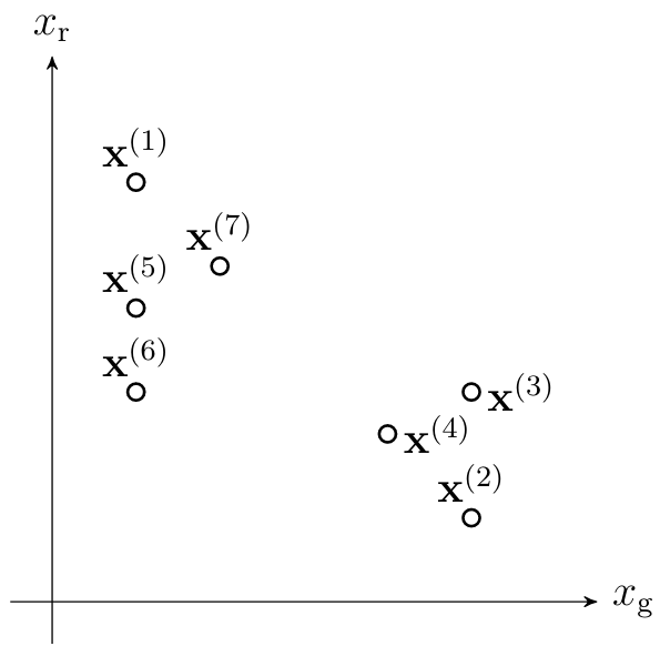
Formally, clustering methods learn a hypothesis that assign each data point either to precisely one cluster (see Section Hard Clustering with kmeans) or several clusters with different degrees of belonging (see Section Soft Clustering with Gaussian Mixture Models ). Different clustering methods use different measures for the similarity between data points. For data points characterized by (numeric) Euclidean feature vectors, the similarity between data points can be naturally defined in terms of the Euclidean distance between feature vectors. Section Connectivity-based Clustering discusses clustering methods that use notions of similarity that are not based on a Euclidean space.
There is a strong conceptual link between clustering methods and the classification methods discussed in Chapter ch_some_examples. Both type of methods learn a hypothesis that reads in the features of a data point and delivers a prediction for some quantity of interest. In classification methods, this quantity of interest is some generic label of a data point. For clustering methods, this quantity of interest for a data point is the cluster assignment (for hard clustering) of the degree of belonging (for soft clustering). A main difference between clustering and classification is that clustering methods do not require the true label (cluster assignment or degree of belonging) of a single data point.
Classification methods learn a good hypothesis via minimizing their average loss incurred on a training set of labeled data points. In contrast, clustering methods do not have access to a single labeled data point. To find the correct labels (cluster assignments) clustering methods rely solely on the intrinsic geometry of the data points. We will see that clustering methods use this intrinsic geometry to define an empirical risk incurred by a candidate hypothesis. Like classification methods, also clustering methods use an instance of the ERM principle (see Chapter Empirical Risk Minimization) to find a good hypothesis (clustering).
This chapter discusses two main flavours of clustering methods:
- hard clustering (see Section Hard Clustering with kmeans)
- and soft clustering methods (see Section Soft Clustering with Gaussian Mixture Models ).
Hard clustering methods learn a hypothesis [math]h[/math] that reads in the feature vector [math]\featurevec[/math] of a data point and delivers a predicted cluster assignment [math]\hat{\truelabel}=h(\featurevec) \in \{1,\ldots,\nrcluster\}[/math]. Thus, assigns each data point to one single cluster. Section Hard Clustering with kmeans will discuss one of the most widely-used hard clustering algorithms which is known as k-means.
In contrast to hard clustering methods, soft clustering methods assign each data point to several clusters with varying degree of belonging. These methods learn a hypothesis that delivers a vector [math]\hat{\labelvec}=\big(\hat{\truelabel}_{1},\ldots,\hat{\truelabel}_{\nrcluster}\big)^{T}[/math] with entry [math]\hat{\truelabel}_{\clusteridx} \in [0,1][/math] being the predicted degree by which the data point belongs to the [math]\clusteridx[/math]-th cluster. Hard clustering is an extreme case of soft clustering where we enforce each degree of belonging to take only values in [math]\{0,1\}[/math]. Moreover, hard clustering requires that for each data point only of the corresponding degree of belonging (one for each cluster) is non-zero.
The main focus of this chapter is on methods that require data points being represented by numeric feature vectors (see Sections Hard Clustering with kmeans and Soft Clustering with Gaussian Mixture Models ). These methods define the similarity between data points using the Euclidean distance between their feature vectors. Some applications generate data points for which it is not obvious how to obtain numeric feature vectors such that their Euclidean distances reflect the similarity between data points. It is then desirable to use a more flexible notion of similarity which does not require to determine (useful) numeric feature vectors of data points.
Maybe the most fundamental concept to represent similarities between data points is a similarity graph. The nodes of the similarity graph are the individual data points of a dataset. Similar data points are connected by edges (links) that might be assigned some weight that quantities the amount of similarity. Section Connectivity-based Clustering discusses clustering methods that use a graph to represent similarities between data points.
Hard Clustering with k-means
Consider a dataset [math]\dataset[/math] which consists of [math]\samplesize[/math] data points that are indexed by [math]\sampleidx=1,\ldots,\samplesize[/math]. The data points are characterized via their numeric feature vectors [math]\featurevec^{(\sampleidx)} \in \mathbb{R}^{\featuredim}[/math], for [math]\sampleidx=1,\ldots,\samplesize[/math]. It will be convenient for the following discussion if we identify a data point with its feature vector. In particular, we refer by [math]\featurevec^{(\sampleidx)}[/math] to the [math]\sampleidx[/math]-th data point. hard clustering methods decompose (or cluster) the dataset into a given number [math]\nrcluster[/math] of different clusters [math]\cluster^{(1)},\ldots,\cluster^{(\nrcluster)}[/math]. These methods assign each data point [math]\featurevec^{(\sampleidx)}[/math] to one and only one cluster [math]\cluster^{(\clusteridx)}[/math] with the cluster index [math]\clusteridx \in \{1,\ldots,\nrcluster\}[/math].
Let us define for each data point its label [math]\truelabel^{(\sampleidx)} \in \{1,\ldots,\nrcluster\}[/math] as the index of the cluster to which the [math]\sampleidx[/math]th data point actually belongs to. The [math]\clusteridx[/math]-th cluster consists of all data points with [math]\truelabel^{(\sampleidx)}=\clusteridx[/math],
We can interpret hard clustering methods as ML methods that compute predictions [math]\hat{\truelabel}^{(\sampleidx)}[/math] for the (“correct”) cluster assignments [math]\truelabel^{(\sampleidx)}[/math]. The predicted cluster assignments result in the predicted clusters
We now discuss a hard clustering method which is known as k-means. This method does not require the knowledge of the label or (true) cluster assignment [math]\truelabel^{(\sampleidx)}[/math] for any data point in [math]\dataset[/math]. This method computes predicted cluster assignments [math]\hat{\truelabel}^{(\sampleidx)}[/math] based solely from the intrinsic geometry of the feature vectors [math]\featurevec^{(\sampleidx)} \in \mathbb{R}^{\featuredim}[/math] for all [math]\sampleidx=1,\ldots,\samplesize[/math]. Since it does not require any labeled data points, k-means is often referred to as being an unsupervised method. However, note that k-means requires the number [math]\nrcluster[/math] of clusters to be given as an input (or hyper-) parameter.
The k-means method represents the [math]\clusteridx[/math]-th cluster [math]\widehat{\cluster}^{(\clusteridx)}[/math] by a representative feature vector [math]\clustermean^{(\clusteridx)} \in \mathbb{R}^{\featuredim}[/math]. It seems reasonable to assign data points in [math]\dataset[/math] to clusters [math]\widehat{\cluster}^{(\clusteridx)}[/math] such that they are well concentrated around the cluster representatives [math]\clustermean^{(\clusteridx)}[/math]. We make this informal requirement precise by defining the clustering error
Note that the clustering error [math]\emperror[/math] \eqref{equ_def_emp_risk_kmeans} depends on both, the cluster assignments [math]\hat{\truelabel}^{(\sampleidx)}[/math], which define the cluster equ_def_individual_cluster, and the cluster representatives [math]\clustermean^{(\clusteridx)}[/math], for [math]\clusteridx=1,\ldots,\nrcluster[/math].
Finding the optimal cluster means [math]\{\clustermean^{(\clusteridx)}\}_{\clusteridx=1}^{\nrcluster}[/math] and cluster assignments [math]\{\hat{\truelabel}^{(\sampleidx)}\}_{\sampleidx=1}^{\samplesize}[/math] that minimize the clustering error \eqref{equ_def_emp_risk_kmeans} is computationally challenging. The difficulty stems from the fact that the clustering error is a non-convex function of the cluster means and assignments. While jointly optimizing the cluster means and assignments is hard, separately optimizing either the cluster means for given assignments or vice-versa is easy. In what follows, we present simple closed-form solutions for these sub-problems. The [math]k[/math]-means method simply combines these solutions in an alternating fashion.
It can be shown that for given predictions (cluster assignments) [math]\hat{\truelabel}^{(\sampleidx)}[/math], the clustering error \eqref{equ_def_emp_risk_kmeans} is minimized by setting the cluster representatives equal to the cluster means
To evaluate \eqref{eq_def_mean_optimal} we need to know the predicted cluster assignments [math]\hat{\truelabel}^{(\sampleidx)}[/math]. The crux is that the optimal predictions [math]\hat{\truelabel}^{(\sampleidx)}[/math], in the sense of minimizing clustering error \eqref{equ_def_emp_risk_kmeans}, depend themselves on the choice for the cluster representatives [math]\clustermean^{(\clusteridx)}[/math]. In particular, for given cluster representative [math]\clustermean^{(\clusteridx)}[/math] with [math]\clusteridx=1,\ldots,\nrcluster[/math], the clustering error is minimized by the cluster assignments
Here, we denote by [math]\argmin\limits_{\clusteridx' \in \{1,\ldots,\nrcluster\}} \| \featurevec^{(\sampleidx)} - \clustermean^{(\clusteridx')} \|[/math] the set of all cluster indices [math]\clusteridx \in \{1,\ldots,\nrcluster\}[/math] such that [math]\| \featurevec^{(\sampleidx)} - \clustermean^{(\clusteridx)} \| = \min_{\clusteridx' \in \{1,\ldots,\nrcluster\}} \| \featurevec^{(\sampleidx)} - \clustermean^{(\clusteridx')} \|[/math].
Note that \eqref{equ_def_clustera_assgt-nearst_mean} assigns the [math]\sampleidx[/math]th datapoint to those cluster [math]\cluster^{(\clusteridx)}[/math] whose cluster mean [math]\clustermean^{(\clusteridx)}[/math] is nearest (in Euclidean distance) to [math]\featurevec^{(\sampleidx)}[/math]. Thus, if we knew the optimal cluster representatives, we could predict the cluster assignments using \eqref{equ_def_clustera_assgt-nearst_mean}. However, we do not know the optimal cluster representatives unless we have found good predictions for the cluster assignments [math]\hat{\truelabel}^{(\sampleidx)}[/math] (see \eqref{eq_def_mean_optimal}).
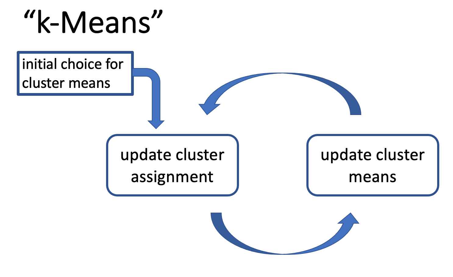
To recap: We have characterized the optimal choice \eqref{eq_def_mean_optimal} for the cluster representatives for given cluster assignments and the optimal choice \eqref{equ_def_clustera_assgt-nearst_mean} for the cluster assignments for given cluster representatives. It seems natural, starting from some initial guess for the cluster representatives, to alternate between the cluster assignment update \eqref{equ_def_clustera_assgt-nearst_mean} and the update \eqref{eq_def_mean_optimal} for the cluster means. This alternating optimization strategy is illustrated in Figure fig_flow_kmeans and summarized in Algorithm k-means. Note that Algorithm k-means, which is maybe the most basic variant of [math]k[/math]-means, simply alternates between the two updates \eqref{eq_def_mean_optimal} and \eqref{equ_def_clustera_assgt-nearst_mean} until some stopping criterion is satisfied.
Algorithm k-means requires the specification of the number [math]\nrcluster[/math] of clusters and initial choices for the cluster means [math]\clustermean^{(\clusteridx)}[/math], for [math]\clusteridx=1,\ldots,\nrcluster[/math]. Those quantities are hyper-parameters that must be tuned to the specific geometry of the given dataset [math]\dataset[/math]. This tuning can be based on probabilistic models for the dataset and its cluster structure (see Section equ_prob_models_data and ). Alternatively, if Algorithm k-means is used as pre-processing within an overall supervised ML method (see Chapter The Landscape of ML), the validation error (see Section sec_modsel) of the overall method might guide the choice of the number [math]\nrcluster[/math] of clusters.
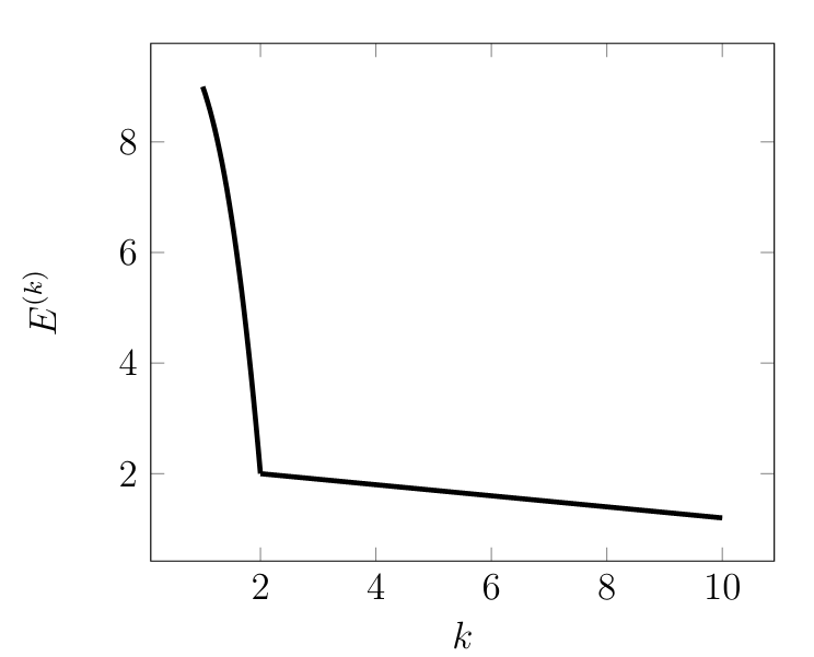
Choosing Number of Clusters. The choice for the number [math]\nrcluster[/math] of clusters typically depends on the role of the clustering method within an overall ML application. If the clustering method serves as a pre-processing for a supervised ML problem, we could try out different values of the number [math]\nrcluster[/math] and determine, for each choice [math]\nrcluster[/math], the corresponding validation error. We then pick the value of [math]\nrcluster[/math] which results in the smallest validation error. If the clustering method is mainly used as a tool for data visualization, we might prefer a small number of clusters. The choice for the number [math]\nrcluster[/math] of clusters can also be guided by the so-called “elbow-method”. Here, we run the [math]k[/math]-means Algorithm k-means for several different choices of [math]\nrcluster[/math]. For each value of [math]\nrcluster[/math], Algorithm k-means delivers a clustering with clustering error
Input: dataset [math]\dataset=\{ \mathbf{x}^{(i)}\}_{i=1}^{n}[/math]; number [math]\nrcluster[/math] of clusters; initial cluster means [math]\clustermean^{(\clusteridx)}[/math] for [math]\clusteridx=1,\ldots,\nrcluster[/math].
- repeat
- for each datapoint [math]\mathbf{x}^{(i)}[/math], [math]i\!=\!1,\ldots,n[/math], do [[math]]\begin{equation}\label{equ_cluster_assign_update} \hat{y}^{(i)} \defeq \argmin\limits_{\clusteridx' \in \{1,\ldots,\nrcluster\}} \| \mathbf{x}^{(i)} - \clustermean^{(\clusteridx')} \| \quad \mbox{ (update cluster assignments)}\end{equation}[[/math]]
- for each cluster [math]\clusteridx\!=\!1,\ldots,\nrcluster[/math] do [[math]]\begin{equation}\label{equ_cluster_mean_update} \clustermean^{(\clusteridx)} \defeq \frac{1}{|\{i: \hat{y}^{(i)}= \clusteridx\}|} \sum_{i: \hat{y}^{(i)} = \clusteridx} \mathbf{x}^{(i)} \quad \mbox{ (update cluster means) }\end{equation}[[/math]]
- until stopping criterion is met
- compute final clustering error [math]\error^{(\nrcluster)} \defeq (1/n) \sum_{i=1}^{n} {\left\|\mathbf{x}^{(i)}-\clustermean^{(\hat{y}^{(i)})}\right\|^2}[/math]
Output: cluster means [math]\clustermean^{(\clusteridx)}[/math], for [math]\clusteridx=1,\ldots,\nrcluster[/math], cluster assignments [math]\hat{y}^{(i)} \in \{1,\ldots,\nrcluster\}[/math], for [math]i=1,\ldots,n[/math], final clustering error [math]\error^{(\nrcluster)}[/math]
We then plot the minimum empirical error [math]\error^{(\nrcluster)}[/math] as a function of the number [math]\nrcluster[/math] of clusters. Figure fig_ellbow depicts an example for such a plot which typically starts with a steep decrease for increasing [math]\nrcluster[/math] and then flattening out for larger values of [math]\nrcluster[/math]. Note that for [math]\nrcluster \geq \samplesize[/math] we can achieve zero clustering error since each datapoint [math]\featurevec^{(\sampleidx)}[/math] can be assigned to a separate cluster [math]\cluster^{(\clusteridx)}[/math] whose mean coincides with that datapoint, [math]\featurevec^{(\sampleidx)} = \clustermean^{(\clusteridx)}[/math].
Cluster-Means Initialization. We briefly mention some popular strategies for choosing the initial cluster means in Algorithm k-means. One option is to initialize the cluster means with realizations of iid random vectors whose probability distribution is matched to the dataset [math]\dataset = \{ \vx^{(\sampleidx)} \}_{\sampleidx=1}^{\samplesize}[/math] (see Section sec_max_iikelihood). For example, we could use a multivariate normal distribution [math]\mathcal{N}(\vx;\widehat{\clustermean}, \widehat{\clustercov})[/math] with the sample mean [math]\widehat{\clustermean} = (1/\samplesize) \sum_{\sampleidx=1}^{\samplesize} \featurevec^{(\sampleidx)}[/math] and the sample covariance [math]\widehat{\clustercov} = (1/\samplesize) \sum_{\sampleidx=1}^{\samplesize} (\featurevec^{(\sampleidx)}\!-\!\widehat{\clustermean}) (\featurevec^{(\sampleidx)}\!-\!\widehat{\clustermean})^{T}[/math]. Alternatively, we could choose the initial cluster means [math]\clustermean^{(\clusteridx)}[/math] by selecting [math]\nrcluster[/math] different data points [math]\featurevec^{(\sampleidx)}[/math] from [math]\dataset[/math]. This selection process might combine random choices with an optimization of the distances between cluster means . Finally, the cluster means might also be chosen by evenly partitioning the principal component of the dataset (see Chapter Feature Learning).
Interpretation as ERM. For a practical implementation of Algorithm k-means we need to decide when to stop updating the cluster means and assignments (see \eqref{equ_cluster_assign_update} and \eqref{equ_cluster_mean_update}). To this end it is useful to interpret Algorithm k-means as a method for iteratively minimizing the clustering error \eqref{equ_def_emp_risk_kmeans}. As can be verified easily, the updates \eqref{equ_cluster_assign_update} and \eqref{equ_cluster_mean_update} always modify (update) the cluster means or assignments in such a way that the clustering error \eqref{equ_def_emp_risk_kmeans} is never increased. Thus, each new iteration of Algorithm k-means results in cluster means and assignments with a smaller (or the same) clustering error compared to the cluster means and assignments obtained after the previous iteration. Algorithm k-means implements a form of ERM (see Chapter Empirical Risk Minimization) using the clustering error \eqref{equ_def_emp_risk_kmeans} as the empirical risk incurred by the predicted cluster assignments [math]\hat{y}^{(\sampleidx)}[/math]. Note that after completing a full iteration of Algorithm k-means, the cluster means [math]\big\{ \clustermean^{(\clusteridx)} \big\}_{\clusteridx=1}^{\nrcluster}[/math] are fully determined by the cluster assignments [math]\big\{ \hat{y}^{(\sampleidx)} \big\}_{\sampleidx=1}^{\samplesize}[/math] via \eqref{equ_cluster_mean_update}. It seems natural to terminate Algorithm k-means if the decrease in the clustering error achieved by the most recent iteration is below a prescribed (small) threshold.
Clustering and Classification. There is a strong conceptual link between Algorithm k-means and classification methods (see e.g. Section sec_nearest_neighbour_methods). Both methods essentially learn a hypothesis [math]h(\featurevec)[/math] that maps the feature vector [math]\featurevec[/math] to a predicted label [math]\hat{\truelabel}=h(\featurevec)[/math] from a finite set. The practical meaning of the label values is different for Algorithm k-means and classification methods. For classification methods, the meaning of the label values is essentially defined by the training set (of labeled data points) used for ERM equ_def_ERM_funs. On the other hand, clustering methods use the predicted label [math]\hat{\truelabel}=h(\featurevec)[/math] as a cluster index.
Another main difference between Algorithm k-means and most classification methods is the choice for the empirical risk used to evaluate the quality or usefulness of a given hypothesis [math]h(\cdot)[/math]. Classification methods typically use an average loss over labeled data points in a training set as empirical risk. In contrast, Algorithm k-means uses the clustering error \eqref{equ_def_emp_risk_kmeans} as a form of empirical risk. Consider a hypothesis that resembles the cluster assignments [math]\hat{\truelabel}^{(\sampleidx)}[/math] obtained after completing an iteration in Algorithm k-means, [math]\hat{\truelabel}^{(\sampleidx)} = h\big( \featurevec^{(\sampleidx)} \big)[/math]. Then we can rewrite the resulting clustering error achieved after this iteration as
Note that the [math]\sampleidx[/math]-th summand in \eqref{equ_emp_risk_clustering} depends on the entire dataset [math]\dataset[/math] and not only on (the features of) the [math]\sampleidx[/math]-th data point [math]\featurevec^{(\sampleidx)}[/math].
Some Practicalities. For a practical implementation of Algorithm k-means we need to fix three issues.
| Issue | Fix |
|---|---|
| Tie-breaking | We need to specify what to do if several different cluster indices [math]\clusteridx\!\in\!\{1,\ldots,\nrcluster\}[/math] achieve the minimum value in the cluster assignment update \eqref{equ_cluster_assign_update} during step equ_step_cluster_asst_update. |
| Empty-cluster | The cluster assignment update \eqref{equ_cluster_assign_update} in step equ_step_cluster_update of Algorithm k-means might result in a cluster [math]\clusteridx[/math] with no datapoints associated with it, [math]|\{ i: \hat{y}^{(i)} = \clusteridx \}|=0[/math]. For such a cluster [math]\clusteridx[/math], the update \eqref{equ_cluster_mean_update} is not well-defined. |
| Stopping-criterion | We need to specify a criterion used in step equ_def_stop_criterion_kmeans of Algorithm k-means to decide when to stop iterating. |
Algorithm k-means II is obtained from Algorithm k-means by fixing those three issues . Step equ_step_cluster_assg_kmeans2 of Algorithm k-means II solves the first issue mentioned above (“tie breaking”), arising when there are several cluster clusters whose means have minimum distance to a data point [math]\featurevec^{(\sampleidx)}[/math], by assigning [math]\vx^{(\sampleidx)}[/math] to the cluster with smallest cluster index (see \eqref{equ_cluster_assign_update2}).
Input: dataset [math]\dataset=\{ \featurevec^{(\sampleidx)}\}_{\sampleidx=1}^{\samplesize}[/math]; number [math]\nrcluster[/math] of clusters; tolerance [math]\varepsilon \geq 0[/math]; initial cluster means [math]\big\{ \clustermean^{(\clusteridx)} \big\}_{\clusteridx=1}^{\nrcluster}[/math]
- Initialize. set iteration counter [math]\itercntr \defeq 0[/math]; [math]\error_{0}\defeq 0[/math]
- repeat
- for all datapoints [math]\sampleidx\!=\!1,\ldots,\samplesize[/math], [[math]]\begin{equation}\label{equ_cluster_assign_update2} \hat{\truelabel}^{(\sampleidx)} \defeq \min \{ \argmin\limits_{\clusteridx' \in \{1,\ldots,\nrcluster\}} \| \featurevec^{(\sampleidx)} - \clustermean^{(\clusteridx')} \| \} \quad \mbox{ (update cluster assignments)}\end{equation}[[/math]]
- for all clusters [math]\clusteridx\!=\!1,\ldots,\nrcluster[/math], update the activity indicator [[math]]b^{(\clusteridx)} \defeq \begin{cases} 1 & \mbox{ if } |\{\sampleidx: \hat{y}^{(\sampleidx)}= \clusteridx\}| \gt 0 \\ 0 & \mbox{ else.} \end{cases}[[/math]]for all [math]\clusteridx\!=\!1,\ldots,\nrcluster[/math] with [math]b^{(\clusteridx)}=1[/math],[[math]]\begin{equation}\label{equ_cluster_mean_update2} \clustermean^{(\clusteridx)} \defeq \frac{1}{|\{ \sampleidx: \hat{\truelabel}^{(\sampleidx)}= \clusteridx\}|} \sum_{\{ \sampleidx: \hat{\truelabel}^{(\sampleidx)} = \clusteridx\}} \featurevec^{(\sampleidx)} \quad \mbox{ (update cluster means) } \end{equation}[[/math]]
- [math]\itercntr \defeq \itercntr+1[/math] (increment iteration counter)
- [math]\error_{\itercntr} \defeq \emperror \big( \{\clustermean^{(\clusteridx)}\}_{\clusteridx=1}^{\nrcluster},\{\hat{\truelabel}^{(\sampleidx)}\}_{\sampleidx=1}^{\samplesize} \mid \dataset \big)[/math] (evaluate clustering error \eqref{equ_def_emp_risk_kmeans})
- [math]\itercntr \gt 1[/math] and [math]\error_{\itercntr\!-\!1} - \error_{\itercntr} \leq \varepsilon[/math] (check for sufficient decrease in clustering error)
- [math]\error^{(\nrcluster)} \defeq (1/\samplesize) \sum_{\sampleidx=1}^{\samplesize} {\left\|\featurevec^{(\sampleidx)}-\clustermean^{(\hat{\truelabel}^{(\sampleidx)})}\right\|^2}[/math] (compute final clustering error)
Output: cluster assignments [math]\hat{\truelabel}^{(\sampleidx)}\!\in\!\{1,\ldots,\nrcluster\}[/math], cluster means [math]\clustermean^{(\clusteridx)}[/math], clustering error [math]\error^{(\nrcluster)}[/math].
Step equ_def_cluster_indicators of Algorithm k-means II resolves the “empty cluster” issue by computing the variables [math]b^{(\clusteridx)} \in \{0,1\}[/math] for [math]\clusteridx=1,\ldots,\nrcluster[/math]. The variable [math]b^{(\clusteridx)}[/math] indicates if the cluster with index [math]\clusteridx[/math] is active ([math]b^{(\clusteridx)}= 1[/math]) or the cluster [math]\clusteridx[/math] is inactive ([math]b^{(\clusteridx)}=0[/math]). The cluster [math]\clusteridx[/math] is defined to be inactive if there are no data points assigned to it during the preceding cluster assignment step \eqref{equ_cluster_assign_update2}. The cluster activity indicators [math]b^{(\clusteridx)}[/math] allows to restrict the cluster mean updates \eqref{equ_cluster_mean_update2} only to the clusters [math]\clusteridx[/math] with at least one data point [math]\featurevec^{(\sampleidx)}[/math]. To obtain a stopping criterion, step equ_def_clustering_error_kmeans2 Algorithm k-means II monitors the clustering error [math]\error_{\itercntr}[/math] incurred by the cluster means and assignments obtained after [math]\itercntr[/math] iterations. Algorithm k-means II continues updating cluster assignments \eqref{equ_cluster_assign_update2} and cluster means \eqref{equ_cluster_mean_update2} as long as the decrease is above a given threshold [math]\varepsilon \geq0[/math].
For Algorithm k-means II to be useful we must ensure that the stopping criterion is met within a finite number of iterations. In other words, we must ensure that the clustering error decrease can be made arbitrarily small within a sufficiently large (but finite) number of iterations. To this end, it is useful to represent Algorithm k-means II as a fixed-point iteration
The operator [math]\mathcal{P}[/math], which depends on the dataset [math]\dataset[/math], reads in a list of cluster assignments and delivers an improved list of cluster assignments aiming at reducing the associated clustering error \eqref{equ_def_emp_risk_kmeans}. Each iteration of Algorithm k-means II updates the cluster assignments [math]\hat{\truelabel}^{(\sampleidx)}[/math] by applying the operator [math]\mathcal{P}[/math]. Representing Algorithm k-means II as a fixed-point iteration \eqref{equ_fixed_point_clustering} allows for an elegant proof of the convergence of Algorithm k-means II within a finite number of iterations (even for [math]\varepsilon = 0[/math]) .
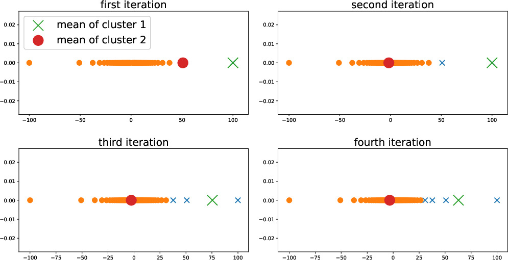
Figure 1.1 depicts the evolution of the cluster assignments and cluster means during the iterations Algorithm k-means II. Each subplot corresponds to one iteration of Algorithm k-means II and depicts the cluster means before that iteration and the clustering assignments (via the marker symbols) after the corresponding iteration. In particular, the upper left subplot depicts the cluster means before the first iteration (which are the initial cluster means) and the cluster assignments obtained after the first iteration of Algorithm k-means II.
Consider running Algorithm k-means II with tolerance [math]\varepsilon=0[/math] (see step step_stop_criterion_kmeans2) such that the iterations are continued until there is no decrease in the clustering error [math]\error^{(\itercntr)}[/math] (see step equ_def_clustering_error_kmeans2 of Algorithm k-means II). As discussed above, Algorithm k-means II will terminate after a finite number of iterations. Moreover, for [math]\varepsilon=0[/math], the delivered cluster assignments [math]\big\{ \hat{\truelabel}^{(\sampleidx)} \big\}_{\sampleidx=1}^{\samplesize}[/math] are fully determined by the delivered clustered means [math]\big\{ \clustermean^{(\clusteridx)} \big\}_{\clusteridx=1}^{\nrcluster}[/math],
Indeed, if \eqref{equ_condition_clusterassmean_kmeans2} does not hold one can show the final iteration [math]r[/math] would still decrease the clustering error and the stopping criterion in step step_stop_criterion_kmeans2 would not be met.
If cluster assignments and cluster means satisfy the condition \eqref{equ_condition_clusterassmean_kmeans2}, we can rewrite the clustering error \eqref{equ_def_emp_risk_kmeans} as a function of the cluster means solely,
Even for cluster assignments and cluster means that do not satisfy \eqref{equ_condition_clusterassmean_kmeans2}, we can still use \eqref{equ_def_clustering_error_means} to lower bound the clustering error \eqref{equ_def_emp_risk_kmeans},
.
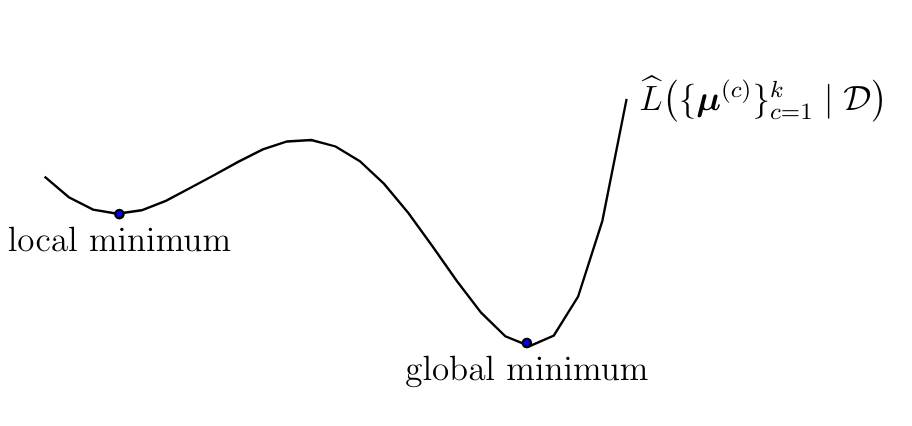
Algorithm k-means II iteratively improves the cluster means in order to minimize \eqref{equ_def_clustering_error_means}. Ideally, we would like Algorithm k-means II to deliver cluster means that achieve the global minimum of \eqref{equ_def_clustering_error_means} (see Figure fig_emp_risk_k_means). However, for some combination of dataset [math]\dataset[/math] and initial cluster means, Algorithm k-means II delivers cluster means that form only a local optimum of [math]\emperror\big( \big\{ \clustermean^{(\clusteridx)} \big\}_{\clusteridx=1}^{\nrcluster} | \dataset \big)[/math] which is strictly worse (larger) than its global optimum (see Figure fig_emp_risk_k_means).
The tendency of Algorithm k-means II to get trapped around a local minimum of \eqref{equ_def_clustering_error_means} depends on the initial choice for cluster means. It is therefore useful to repeat Algorithm k-means II several times, with each repetition using a different initial choice for the cluster means. We then pick the cluster assignments [math]\{ \hat{\truelabel}^{(\sampleidx)} \}_{\sampleidx=1}^{\samplesize}[/math] obtained for the repetition that resulted in the smallest clustering error [math]\error^{(\nrcluster)}[/math] (see step equ_def_step_final_clustering_kmeans2).
Soft Clustering with Gaussian Mixture Models
Consider a dataset [math]\dataset=\{\featurevec^{(1)},\ldots,\featurevec^{(\samplesize)}\}[/math] that we wish to group into a given number of [math]\nrcluster[/math] different clusters. The hard clustering methods discussed in Section Hard Clustering with kmeans deliver cluster assignments [math]\hat{\truelabel}^{(\sampleidx)}[/math], for [math]\sampleidx=1,\ldots,\samplesize[/math]. The cluster assignment [math]\hat{\truelabel}^{(\sampleidx)}[/math] is the index of the cluster to which the [math]\sampleidx[/math]th data point [math]\featurevec^{(\sampleidx)}[/math] is assigned to. These cluster assignments [math]\hat{\truelabel}[/math] provide rather coarse-grained information. Two data points [math]\featurevec^{(\sampleidx)}, \featurevec^{(\sampleidx')}[/math] might be assigned to the same cluster [math]\clusteridx[/math] although their distances to the cluster mean [math]\clustermean^{(\clusteridx)}[/math] might differ significantly. Intuitively, these two data points have a different degree of belonging to the cluster [math]\clusteridx[/math].
For some clustering applications it is desirable to quantify the degree by which a data point belongs to a cluster. Soft clustering methods use a continues range, such as the closed interval [math][0,1][/math], of possible values for the degree of belonging. In contrast, hard clustering methods use only two possible values for the degree of belonging to a specific cluster, either “full belonging” or no “belonging at all”. While hard clustering methods assign a given data point to precisely one cluster, soft clustering methods typically assign a data point to several different clusters with non-zero degree of belonging.
This chapter discusses soft clustering methods that compute, for each data point [math]\featurevec^{(\sampleidx)}[/math] in the dataset [math]\dataset[/math], a vector [math]\widehat{\labelvec}^{(\sampleidx)}=\big(\hat{\truelabel}_{1}^{(\sampleidx)},\ldots,\hat{\truelabel}_{\nrcluster}^{(\sampleidx)}\big)^{T}[/math]. We can interpret the entry [math]\hat{\truelabel}_{\clusteridx}^{(\sampleidx)} \in [0,1][/math] as the degree by which the data point [math]\featurevec^{(\sampleidx)}[/math] belongs to the cluster [math]\cluster^{(\clusteridx)}[/math]. For [math]\hat{\truelabel}_{\clusteridx}^{(\sampleidx)} \approx 1[/math], we are quite confident in the data point [math]\featurevec^{(\sampleidx)}[/math] belonging to cluster [math]\cluster^{(\clusteridx)}[/math]. In contrast, for [math]\hat{\truelabel}_{\clusteridx}^{(\sampleidx)} \approx 0[/math], we are quite confident that the data point [math]\featurevec^{(\sampleidx)}[/math] is outside the cluster [math]\cluster^{(\clusteridx)}[/math].
A widely used soft clustering method uses a probabilistic model for the data points [math]\dataset = \{ \featurevec^{(\sampleidx)} \}_{\sampleidx=1}^{\samplesize}[/math]. Within this model, each cluster [math]\cluster^{(\clusteridx)}[/math], for [math]\clusteridx=1,\ldots,\nrcluster[/math], is represented by a multivariate normal distribution
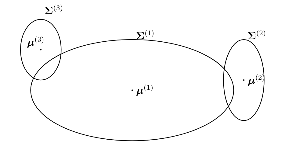
The probability distribution \eqref{equ_def_mvn_distribution} is parametrized by a cluster-specific mean vector [math]\clustermean^{(\clusteridx)}[/math] and an (invertible) cluster-specific covariance matrix [math]\clustercov^{(\clusteridx)}[/math].[1] Let us interpret a specific data point [math]\featurevec^{(\sampleidx)}[/math] as a realization drawn from the probability distribution \eqref{equ_def_mvn_distribution} of a specific cluster [math]\clusteridx^{(\sampleidx)}[/math],
We can think of [math]\clusteridx^{(\sampleidx)}[/math] as the true index of the cluster to which the data point [math]\featurevec^{(\sampleidx)}[/math] belongs to. The variable [math]\clusteridx^{(\sampleidx)}[/math] selects the cluster distributions \eqref{equ_def_mvn_distribution} from which the feature vector [math]\featurevec^{(\sampleidx)}[/math] has been generated (drawn). We will therefore refer to the variable [math]\clusteridx^{(\sampleidx)}[/math] as the (true) cluster assignment for the [math]\sampleidx[/math]th data point. Similar to the feature vectors [math]\featurevec^{(\sampleidx)}[/math] we also interpret the cluster assignments [math]\clusteridx^{(\sampleidx)}[/math], for [math]\sampleidx=1,\ldots,\samplesize[/math] as realizations of iid rvs.
In contrast to the feature vectors [math]\featurevec^{(\sampleidx)}[/math], we do not observe (know) the true cluster indices [math]\clusteridx^{(\sampleidx)}[/math]. After all, the goal of soft clustering is to estimate the cluster indices [math]\clusteridx^{(\sampleidx)}[/math]. We obtain a soft clustering method by estimating the cluster indices [math]\clusteridx^{(\sampleidx)}[/math] based solely on the data points in [math]\dataset[/math]. To compute these estimates we assume that the (true) cluster indices [math]\clusteridx^{(\sampleidx)}[/math] are realizations of iid rvs with the common probability distribution (or probability mass function)
The (prior) probabilities [math]p_{\clusteridx}[/math], for [math]\clusteridx=1,\ldots,\nrcluster[/math], are either assumed known or estimated from data . The choice for the probabilities [math]p_{\clusteridx}[/math] could reflect some prior knowledge about different sizes of the clusters. For example, if cluster [math]\cluster^{(1)}[/math] is known to be larger than cluster [math]\cluster^{(2)}[/math], we might choose the prior probabilities such that [math]p_{1} \gt p_{2}[/math].
The probabilistic model given by \eqref{equ_cond_dist_GMM}, \eqref{equ_def_cluster_prob} is referred to as a GMM. This name is quite natural as the common marginal distribution for the feature vectors [math]\featurevec^{(\sampleidx)}[/math], for [math]\sampleidx=1,\ldots,\samplesize[/math], is a (additive) mixture of multivariate normal (Gaussian) distributions,
As already mentioned, the cluster assignments [math]\clusteridx^{(\sampleidx)}[/math] are hidden (unobserved) rvs. We thus have to infer or estimate these variables from the observed data points [math]\featurevec^{(\sampleidx)}[/math] which realizations or iid rvs with the common distribution \eqref{equ_def_GMM}.
The GMM (see \eqref{equ_cond_dist_GMM} and \eqref{equ_def_cluster_prob}) lends naturally to a rigorous definition for the degree [math]\truelabel^{(\sampleidx)}_{\clusteridx}[/math] by which data point [math]\featurevec^{(\sampleidx)}[/math] belongs to cluster [math]\clusteridx[/math].[2] Let us define the label value [math]\truelabel^{(\sampleidx)}_{\clusteridx}[/math] as the “a-posteriori” probability of the cluster assignment [math]\clusteridx^{(\sampleidx)}[/math] being equal to [math]\clusteridx \in \{1,\ldots,\nrcluster\}[/math]:
By their very definition \eqref{equ_def_deg_belonging_prob}, the degrees of belonging [math]y^{(\sampleidx)}_{\clusteridx}[/math] always sum to one,
We emphasize that we use the conditional cluster probability \eqref{equ_def_deg_belonging_prob}, conditioned on the dataset [math]\dataset[/math], for defining the degree of belonging [math]\truelabel^{(\sampleidx)}_{\clusteridx}[/math]. This is reasonable since the degree of belonging [math]\truelabel^{(\sampleidx)}_{\clusteridx}[/math] depends on the overall (cluster) geometry of the dataset [math]\dataset[/math].
The definition \eqref{equ_def_deg_belonging_prob} for the label values (degree of belongings) [math]\truelabel^{(\sampleidx)}_{\clusteridx}[/math] involves the GMM parameters [math]\{\clustermean^{(\clusteridx)},\clustercov^{(\clusteridx)},p_{\clusteridx}\}_{\clusteridx=1}^{\nrcluster}[/math] (see \eqref{equ_def_GMM}). Since we do not know these parameters beforehand we cannot evaluate the conditional probability in \eqref{equ_def_deg_belonging_prob}. A principled approach to solve this problem is to evaluate \eqref{equ_def_deg_belonging_prob} with the true GMM parameters replaced by some estimates [math]\{\widehat{\clustermean}^{(\clusteridx)},\widehat{\clustercov}^{(\clusteridx)},\hat{p}_{\clusteridx}\}_{\clusteridx=1}^{\nrcluster}[/math]. Plugging in the GMM parameter estimates into \eqref{equ_def_deg_belonging_prob} provides us with predictions [math]\hat{\truelabel}^{(\sampleidx)}_{\clusteridx}[/math] for the degrees of belonging. However, to compute the GMM parameter estimates we would have already needed the degrees of belonging [math]\truelabel^{(\sampleidx)}_{\clusteridx}[/math]. This situation is similar to hard clustering where ultime goals is to jointly optimize cluster means and assignments (see Section Hard Clustering with kmeans).
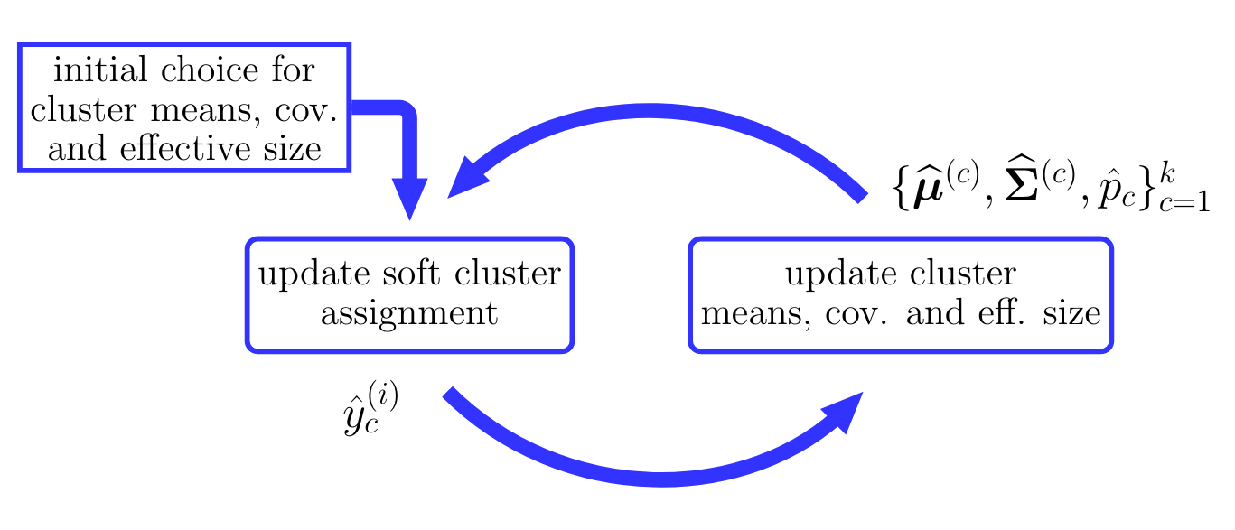
Similar to the spirit of Algorithm k-means for hard clustering, we solve the above dilemma of soft clustering by an alternating optimization scheme. This scheme, which is illustrated in Figure fig_flow_softclustering, alternates between updating (optimizing) the predicted degrees of belonging (or soft cluster assignments) [math]\hat{\truelabel}^{(\sampleidx)}_{\clusteridx}[/math], for [math]\sampleidx=1,\ldots,\samplesize[/math] and [math]\clusteridx=1,\ldots,\nrcluster[/math], given the current GMM parameter estimates [math]\{\widehat{\clustermean}^{(\clusteridx)},\widehat{\clustercov}^{(\clusteridx)},\hat{p}_{\clusteridx}\}_{\clusteridx=1}^{\nrcluster}[/math] and then updating (optimizing) these GMM parameter estimates based on the updated predictions [math]\hat{\truelabel}^{(\sampleidx)}_{\clusteridx}[/math]. We summarize the resulting soft clustering method in Algorithm Soft-Clustering Algorithm. Each iteration of Algorithm Soft-Clustering Algorithm consists of an update \eqref{equ_update_soft_cluster_assignm} for the degrees of belonging followed by an update (step equ_GMM_update_step) for the GMM parameters.
To analyze Algorithm Soft-Clustering Algorithm it is helpful to interpret (the features of) data points [math]\featurevec^{(\sampleidx)}[/math] as realizations of iid rvs distributed according to a GMM \eqref{equ_cond_dist_GMM}-\eqref{equ_def_cluster_prob}. We can then understand Algorithm Soft-Clustering Algorithm as a method for estimating the GMM parameters based on observing realizations drawn from the GMM \eqref{equ_cond_dist_GMM}-\eqref{equ_def_cluster_prob}. We can estimate the parameters of a probability distribution using the maximum likelihood method (see Section sec_max_iikelihood and ). As its name suggests, maximum likelihood methods estimate the GMM parameters by maximizing the probability (density)
of actually observing the data points in the dataset [math]\dataset[/math].
It can be shown that Algorithm Soft-Clustering Algorithm is an instance of a generic approximate maximum likelihood technique referred to as expectation maximization EM (see for more details). In particular, each iteration of Algorithm Soft-Clustering Algorithm updates the GMM parameter estimates such that the corresponding probability density \eqref{equ_def_prob_den_GMM} does not decrease . If we denote the GMM parameter estimate obtained after [math]\itercntr[/math] iterations of Algorithm Soft-Clustering Algorithm by [math]{\boldsymbol \theta}^{(\itercntr)}[/math] ,
Input: dataset [math]\dataset=\{ \featurevec^{(\sampleidx)}\}_{\sampleidx=1}^{\samplesize}[/math]; number [math]\nrcluster[/math] of clusters, initial GMM parameter estimates [math]\{\widehat{\clustermean}^{(\clusteridx)},\widehat{\clustercov}^{(\clusteridx)},\hat{p}_{\clusteridx}\}_{\clusteridx=1}^{\nrcluster}[/math]
- repeat
- for each [math]\sampleidx=1,\ldots,\samplesize[/math] and [math]\clusteridx=1,\ldots,\nrcluster[/math], update degrees of belonging [[math]]\begin{align} \label{equ_update_soft_cluster_assignm} \hat{\truelabel}_{\clusteridx}^{(\sampleidx)} & \defeq \frac{\hat{p}_{\clusteridx} \mathcal{N}(\featurevec^{(\sampleidx)};\widehat{\clustermean}^{(\clusteridx)},\widehat{\clustercov}^{(\clusteridx)})}{\sum_{\clusteridx'=1}^{\nrcluster} \hat{p}_{\clusteridx'}\mathcal{N}(\featurevec^{(\sampleidx)};\widehat{\clustermean}^{(\clusteridx')},\widehat{\clustercov}^{(\clusteridx')})} %\nonumber \\ \end{align}[[/math]]
- for each [math]\clusteridx \in \{1,\ldots,\nrcluster\}[/math], update GMM parameter estimates:
- [math]\hat{p}_{\clusteridx}\!\defeq\!\samplesize_{\clusteridx} /\samplesize[/math] with effective cluster size [math]\samplesize_{\clusteridx} \defeq \sum\limits_{\sampleidx=1}^{\samplesize} \hat{\truelabel}_{\clusteridx}^{(\sampleidx)}[/math] (cluster probability)
- [math]\widehat{\clustermean}^{(\clusteridx)} \defeq (1/\samplesize_{\clusteridx}) \sum\limits_{\sampleidx=1}^{\samplesize} \hat{\truelabel}_{\clusteridx}^{(\sampleidx)} \featurevec^{(\sampleidx)}[/math] (cluster mean)
- [math]\widehat{\clustercov}^{(\clusteridx)} \defeq (1/\samplesize_{\clusteridx}) {\sum\limits_{\sampleidx=1}^{\samplesize} \hat{\truelabel}_{\clusteridx}^{(\sampleidx)} \big(\featurevec^{(\sampleidx)}\!-\!\widehat{\clustermean}^{(\clusteridx)}\big) \big(\featurevec^{(\sampleidx)}\!-\!\widehat{\clustermean}^{(\clusteridx)}\big)^{T} }[/math] (cluster covariance matrix)
- until stopping criterion met
Output: predicted degrees of belonging [math]\widehat{\labelvec}^{(\sampleidx)}=(\hat{\truelabel}_{1}^{(\sampleidx)},\ldots,\hat{y}_{\nrcluster}^{(\sampleidx)})^{T}[/math] for [math]\sampleidx=1,\ldots,\samplesize[/math].
As for Algorithm k-means, we can also interpret Algorithm Soft-Clustering Algorithm as an instance of the ERM principle discussed in Chapter ch_Optimization. Indeed, maximizing the probability density \eqref{equ_def_prob_den_GMM} is equivalent to minimizing the empirical risk
The empirical risk \eqref{equ_def_emp_risk_soft_clustering} is the negative logarithm of the probability (density) \eqref{equ_def_prob_den_GMM} of observing the dataset [math]\dataset[/math] as iid realizations of the GMM \eqref{equ_def_GMM}. The monotone increase in the probability density \eqref{equ_proability_increasing_GMM} achieved by the iterations of Algorithm Soft-Clustering Algorithm translate into a monotone decrease of the empirical risk,
The monotone decrease \eqref{equ_emprisk_decreasing_GMM} in the empirical risk \eqref{equ_def_emp_risk_soft_clustering} achieved by the iterations of Algorithm Soft-Clustering Algorithm naturally lends to a stopping criterion. Let [math]\error_{\itercntr}[/math] denote the empirical risk \eqref{equ_def_emp_risk_soft_clustering} achieved by the GMM parameter estimates [math]{\boldsymbol \theta}^{(\itercntr)}[/math] obtained after [math]\itercntr[/math] iterations in Algorithm Soft-Clustering Algorithm. Algorithm Soft-Clustering Algorithm stops iterating as soon as the decrease [math]\error_{\itercntr\!-\!1} - \error_{\itercntr}[/math] achieved by the [math]\itercntr[/math]-th iteration of Algorithm Soft-Clustering Algorithm falls below a given (positive) threshold [math]\varepsilon\gt0[/math].
Similar to Algorithm k-means, also Algorithm Soft-Clustering Algorithm might get trapped in local minima of the underlying empirical risk. The GMM parameters delivered by Algorithm Soft-Clustering Algorithm might only be a local minimum of \eqref{equ_def_emp_risk_soft_clustering} but not the global minimum (see Figure fig_emp_risk_k_means for the analogous situation in hard clustering). As for hard clustering Algorithm k-means, we typically repeat Algorithm Soft-Clustering Algorithm several times. During each repetition of Algorithm Soft-Clustering Algorithm, we use a different (randomly chosen) initialization for the GMM parameter estimates [math]{\boldsymbol \theta} = \{ \widehat{\clustermean}^{(\clusteridx)}, \widehat{\clustercov}^{(\clusteridx)}, \hat{p}_{\clusteridx} \}_{\clusteridx=1}^{\nrcluster}[/math]. Each repetition of Algorithm Soft-Clustering Algorithm results in a potentially different set of GMM parameter estimates and degrees of belongings [math]\hat{y}^{(\sampleidx)}_{\clusteridx}[/math]. We then use the results for that repetition that achieves the smallest empirical risk \eqref{equ_def_emp_risk_soft_clustering}.
Let us point out an interesting link between soft clustering methods based on GMM (see Algorithm Soft-Clustering Algorithm) and hard clustering with k-means (see Algorithm k-means). Consider the GMM \eqref{equ_cond_dist_GMM} with prescribed cluster covariance matrices
with some given variance [math]\sigma^{2}\gt0[/math]. We assume the cluster covariance matrices in the GMM to be given by \eqref{equ_def_special_case} and therefore can replace the covariance matrix updates in Algorithm Soft-Clustering Algorithm with the assignment [math]\widehat{\clustercov}^{(\clusteridx)} \defeq \sigma^{2} \mathbf{I}[/math]. It can be verified easily that for sufficiently small variance [math]\sigma^{2}[/math] in \eqref{equ_def_special_case}, the update \eqref{equ_update_soft_cluster_assignm} tends to enforce [math]\hat{y}_{\clusteridx}^{(\sampleidx)} \in \{0,1\}[/math]. In other words, each data point [math]\featurevec^{(\sampleidx)}[/math] becomes then effectively associated with exactly one single cluster [math]\clusteridx[/math] whose cluster mean [math]\widehat{\clustermean}^{(\clusteridx)}[/math] is nearest to [math]\featurevec^{(\sampleidx)}[/math]. For [math]\sigma^{2} \rightarrow 0[/math], the soft clustering update \eqref{equ_update_soft_cluster_assignm} in Algorithm Soft-Clustering Algorithm reduces to the (hard) cluster assignment update \eqref{equ_cluster_assign_update} in k-means Algorithm k-means. We can interpret Algorithm k-means as an extreme case of Algorithm Soft-Clustering Algorithm that is obtained by fixing the covariance matrices in the GMM to [math]\sigma^{2} \mathbf{I}[/math] with a sufficiently small [math]\sigma^{2}[/math].
Combining GMM with linear regression. Let us sketch how Algorithm Soft-Clustering Algorithm could be combined with linear regression methods (see Section sec_lin_reg). The idea is to first compute the degree of belongings to the clusters for each data point. We then learn separate linear predictors for each cluster using the degree of belongings as weights for the individual loss terms in the training error. To predict the label of a new data point, we first compute the predictions obtained for each cluster-specific linear hypothesis. These cluster-specific predictions are then averaged using the degree of belongings for the new data point as weights.
Connectivity-based Clustering
The clustering methods discussed in Sections Hard Clustering with kmeans and Soft Clustering with Gaussian Mixture Models can only be applied to data points which are characterized by numeric feature vectors. These methods define the similarity between data points using the Euclidean distance between the feature vectors of these data points. As illustrated in Figure fig_GMM_kmeans_geometry, these methods can only produce “Euclidean shaped” clusters that are contained either within hyper-spheres (Algorithm k-means) or hyper-ellipsoids (Algorithm Soft-Clustering Algorithm).

Some applications generate data points for which the construction of useful numeric features is difficult. Even if we can easily obtain numeric features for data points, the Euclidean distances between the resulting feature vectors might not reflect the actual similarities between data points. As a case in point, consider data points representing text documents. We could use the histogram of a respecified list of words as numeric features for a text document. In general, a small Euclidean distance between histograms of text documents does not imply that the text documents have similar meanings. Moreover, clusters of similar text documents might have highly complicated shapes in the space of feature vectors that cannot be grouped within hyper-ellipsoids. For datasets with such “non-Euclidean” cluster shapes, k-means or GMM are not suitable as clustering methods. We should then replace the Euclidean distance between feature vectors with another concept to determine or measure the similarity between data points.
Connectivity-based clustering methods do not require any numeric features of data points. These methods cluster data points based on explicitly specifying for any two different data points if they are similar and to what extend. A convenient mathematical tool to represent similarities between the data points of a dataset [math]\dataset[/math] is a weighted undirected graph [math]\graph=\big(\nodes,\edges\big)[/math]. We refer to this graph as the similarity graph of the dataset [math]\dataset[/math] (see Figure fig_connect_clustering). The nodes [math]\nodes[/math] in this similarity graph [math]\graph[/math] represent data points in [math]\dataset[/math] and the undirected edges connect nodes that represent similar data points. The extend of the similarity is represented by the weights [math]W_{\nodeidx,\nodeidx'}[/math] for each edge [math]\{\nodeidx,\nodeidx'\} \in \edges[/math].
Given a similarity graph [math]\graph[/math] of a dataset, connectivity-based clustering methods determine clusters as subsets of nodes that are well connected within the cluster but weakly connected between different clusters. Different concepts for quantifying the connectivity between nodes in a graph yield different clustering methods. Spectral clustering methods use eigenvectors of a graph Laplacian matrix to measure the connectivity between nodes . Flow-based clustering methods measure the connectivity between two nodes via the amount of flow that can be routed between them . Note that we might use these connectivity measures to construct meaningful numerical feature vectors for the nodes in the empirical graph. These feature vectors can then be fed into the hard-clustering Algorithm k-means II or the soft clustering Algorithm Soft-Clustering Algorithm (see Figure fig_connect_clustering).
The algorithm DBSCAN considers two data points [math]\sampleidx,\sampleidx'[/math] as connected if one of them (say [math]\sampleidx[/math]) is a core node and the other node ([math]\sampleidx'[/math]) can be reached via a sequence (path) of connected core nodes
DBSCAN considers a node to be a core node if it has a sufficiently large number of neighbours . The minimum number of neighbours required for a node to be considered a core node is a hyper-parameter of DBSCAN. When DBSCAN is applied to data points with numeric feature vectors, it defines two data points as connected if the Euclidean distance between their feature vectors does not exceed a given threshold [math]\varepsilon[/math] (see Figure fig_DBSCAN).
In contrast to k-means and GMM, DBSCAN does not require the number of clusters to be specified. The number of clusters is determined automatically by DBSCAN and depends on its hyper-parameters. DBSCAN also performs an implicit outlier detection. The outliers delivered by DBSCAN are those data points which do not belong to the same cluster as any other data point.
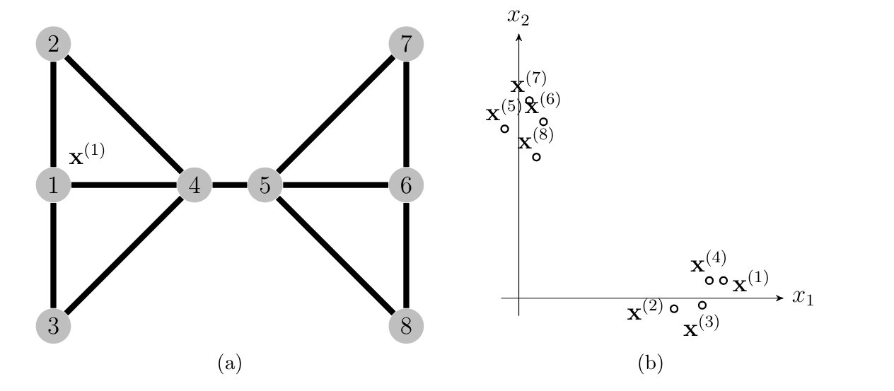
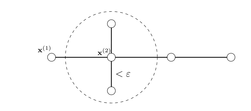
Clustering as Preprocessing
In applications it might be benefiial to combine clustering methods with supervised methods such as linear regression. As a point in case consider a dataset that consists of data points obtained from two different data generation processes. Let us denote the data points generated by one process by [math]\dataset^{(1)}[/math] and the other one by [math]\dataset^{(2)}[/math]. Each datapoint is characterzed by features and a label. While there would be an accurate lienar hypothesis for predicting the label of datapoints in [math]\dataset^{(1)}[/math] and another linear hypothesis for [math]\dataset^{(2)}[/math] these two are very different.
We could try to use clustering methods to assign any given data point to the corresponding data generation process. If we are lucky, the resulting clusters resemble (approximately) the two data generation processes [math]\dataset^{(1)}[/math] and [math]\dataset^{(2)}[/math]. Once we have successfully clustered the data points, we can learn a separate (tailored) hypothesis for ach cluster. More generally, we can use the predicted cluster assignments obtained from the methods of Section Hard Clustering with kmeans - Connectivity-based Clustering as additional features for each data point.
Let us illustrate the above ideas by combining Algorithm k-means with linear regression. We first group data points into a given number [math]\nrcluster[/math] of clusters and then learn separate linear predictors [math]h^{(\clusteridx)}(\featurevec)=\big( \weights^{(\clusteridx)} \big)^{T} \featurevec[/math] for each cluster [math]\clusteridx=1,\ldots,\nrcluster[/math]. To predict the label of a new data point with features [math]\featurevec[/math], we first assign to the cluster [math]\clusteridx'[/math] with the nearest cluster mean. We then use the linear predictor [math]h^{(\clusteridx')}[/math] assigned to cluster [math]\clusteridx'[/math] to compute the predicted label [math]\hat{\truelabel} = h^{(\clusteridx')}(\featurevec)[/math].
Notes
- Note that the expression \eqref{equ_def_mvn_distribution} is only valid for an invertible (non-singular) covariance matrix [math]\clustercov[/math].
- Remember that the degree of belonging [math]\truelabel^{(\sampleidx)}_{\clusteridx}[/math] is considered as the (unknown) label value of a data point. The choice or definition for the labels of data points is a design choice. In particular, we can define the labels of data points using a hypothetical probabilistic model such as the GMM.
References
Jung, Alexander (2022). Machine Learning: The Basics. Signapore: Springer. doi:10.1007/978-981-16-8193-6.
Jung, Alexander (2022). "Machine Learning: The Basics". arXiv:1805.05052.