guide:352d094fa1

[math] \newcommand{\ex}[1]{\item } \newcommand{\sx}{\item} \newcommand{\x}{\sx} \newcommand{\sxlab}[1]{} \newcommand{\xlab}{\sxlab} \newcommand{\prov}[1] {\quad #1} \newcommand{\provx}[1] {\quad \mbox{#1}} \newcommand{\intext}[1]{\quad \mbox{#1} \quad} \newcommand{\R}{\mathrm{\bf R}} \newcommand{\Q}{\mathrm{\bf Q}} \newcommand{\Z}{\mathrm{\bf Z}} \newcommand{\C}{\mathrm{\bf C}} \newcommand{\dt}{\textbf} \newcommand{\goesto}{\rightarrow} \newcommand{\ddxof}[1]{\frac{d #1}{d x}} \newcommand{\ddx}{\frac{d}{dx}} \newcommand{\ddt}{\frac{d}{dt}} \newcommand{\dydx}{\ddxof y} \newcommand{\nxder}[3]{\frac{d^{#1}{#2}}{d{#3}^{#1}}} \newcommand{\deriv}[2]{\frac{d^{#1}{#2}}{dx^{#1}}} \newcommand{\dist}{\mathrm{distance}} \newcommand{\arccot}{\mathrm{arccot\:}} \newcommand{\arccsc}{\mathrm{arccsc\:}} \newcommand{\arcsec}{\mathrm{arcsec\:}} \newcommand{\arctanh}{\mathrm{arctanh\:}} \newcommand{\arcsinh}{\mathrm{arcsinh\:}} \newcommand{\arccosh}{\mathrm{arccosh\:}} \newcommand{\sech}{\mathrm{sech\:}} \newcommand{\csch}{\mathrm{csch\:}} \newcommand{\conj}[1]{\overline{#1}} \newcommand{\mathds}{\mathbb} [/math]

The straight-line distance in the plane between two points [math]P = (x_1, y_1)[/math] and [math]Q = (x_2, y_2)[/math] is defined in Section 2 of Chapter 1 by the formula

[[math]] \begin{equation} distance(P, Q) = \sqrt{(x_2 - x_1)^2 + (y_2 - y_1)^2} . \label{eq10.2.1} \end{equation} [[/math]]

In this section we shall consider the harder problem of defining distance, or arc length, along a parametrized curve. Let [math]C[/math] be a curve parametrically defined by a continuous function [math]P: I \rightarrow R^2[/math], and let [math]a[/math] and [math]b[/math] be two numbers in the interval [math]I[/math] such that [math]a \lt b[/math]. As we have seen in Section \secref{10.1}, [math]C[/math] is the set of all points

[[math]] P(t) = (x(t), y(t)), \;\;\;\mbox{for every $t$ in $I$.} [[/math]]

Consider a partition [math]\sigma = \{ t_0, . . . , t_n \}[/math] of the closed interval [math][a, b][/math] such that

[[math]] a = t_0 \leq t_1 \leq \cdots \leq t_n = b, [[/math]]

and set [math]P(t_i) = P_i[/math], for every [math]i = 0, . . ., n[/math]. We shall take the number [math]L_\sigma[/math] defined by

[[math]] \begin{equation} L_\sigma = \sum_{i=1}^n distance (P_{i-1}, P_i) \label{eq10.2.2} \end{equation} [[/math]]

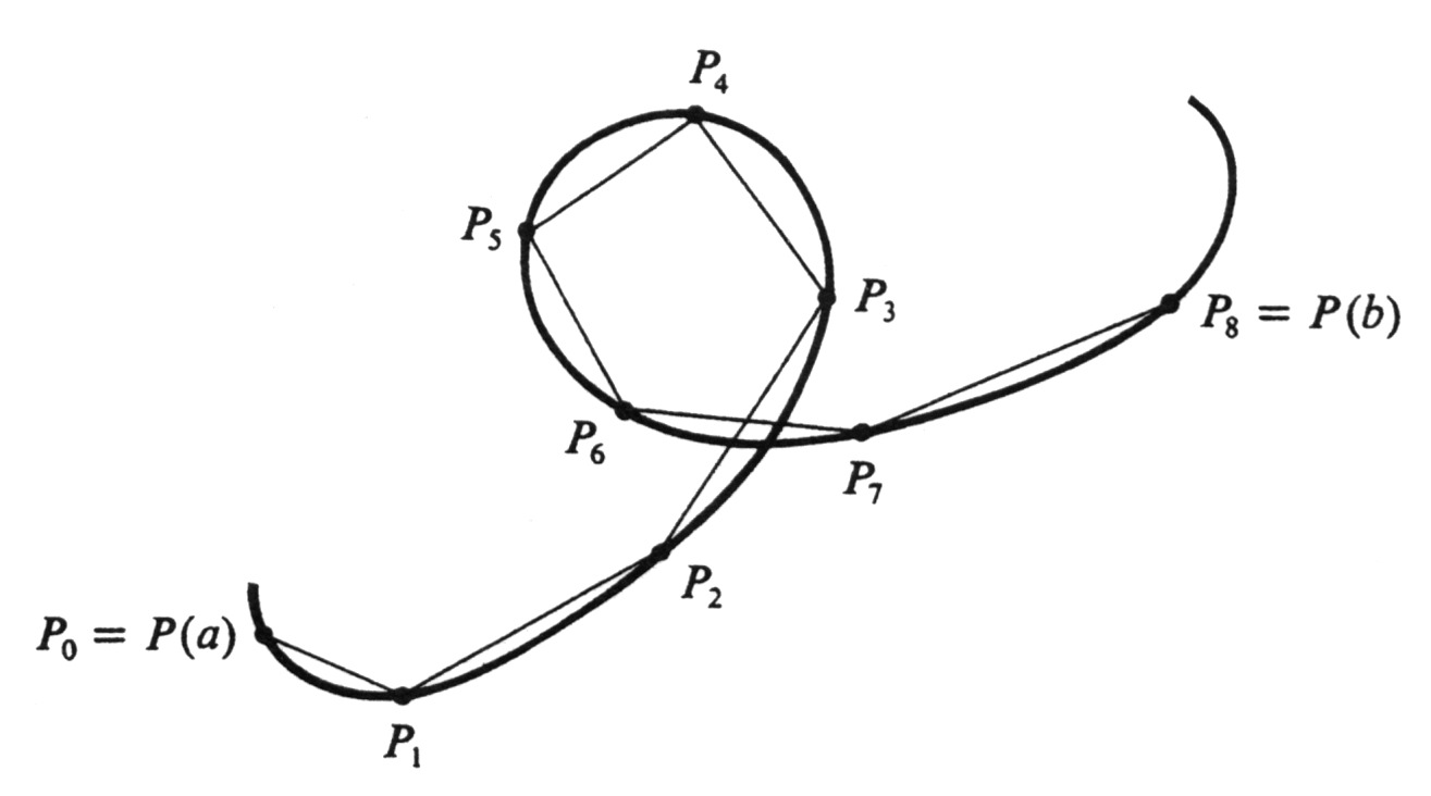
as an approximation to the arc length along [math]C[/math] from [math]P(a)[/math] to [math]P(b)[/math]. In Figure 6, the number [math]L_\sigma[/math] is the sum of the lengths of the straight-line segments joining the points along the curve. Using (1), we may also write

[[math]] L_\sigma = \sum_{i=1}^n \sqrt{[x(t_i) - x(t_{i-1})]^2 + [y(t_i) - y(t_{i-1})]^2} . [[/math]]

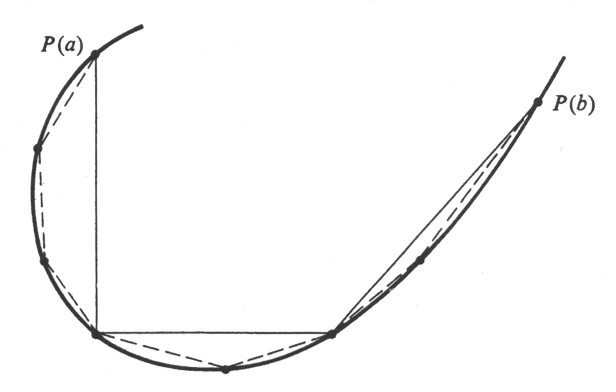
The principle which motivates the definition of arc length is the fact that if one partition [math]\sigma[/math] of [math][a, b][/math] is a subset of another partition [math]\tau[/math], then [math]L_\tau[/math] is in general a better approximation than [math]L_\sigma[/math]. The basic reason for this is simply that the finer partition [math]\tau[/math] determines more points on the curve. As an example, consider Figure 7, in which [math]L_\sigma[/math] is the sum of the lengths of the solid straightline segments, and [math]L_\tau[/math] is the sum of the lengths of the dashed-line segments. It is clear from the picture that [math]L_\tau[/math] is closer than [math]L_\sigma[/math] to our intuitive idea of the arc length of the curve. Moreover,

Theorem

If one partition [math]\sigma[/math] of [math][a, b][/math] is a subset of another [math]\tau[/math], then [math]L_\sigma \leq L_\tau[/math].

Show Proof

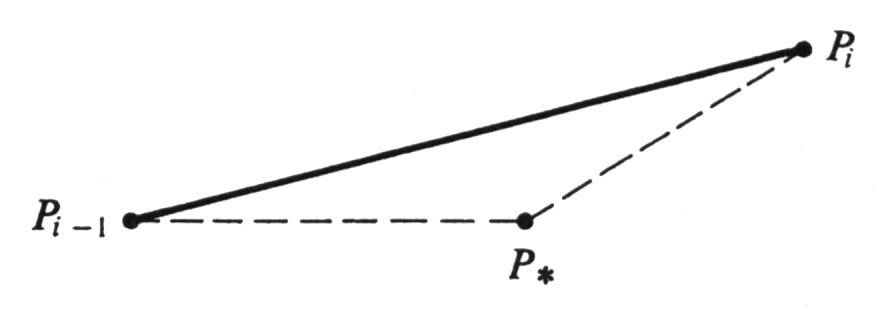
This fact is geometrically apparent from Figure 7. The argument can be reduced to consideration of a single triangle by the realization that, since [math]\tau[/math] can be obtained from [math]\sigma[/math] by adjoining one new point at a time, it will be sufficient to prove the result under the assumption that [math]\tau[/math] differs from [math]\sigma[/math] by the inclusion of only one additional point, which we denote by [math]t_{*}[/math]. Let [math]P_{*} = P(t_{*})[/math]. For some integer [math]i[/math], we have [math]t_{i-1} \lt t_{*} \lt t_i[/math]. Then the expressions for [math]L_\sigma[/math] and [math]L_\tau[/math] are obviously the same except that the term [math]distance(P_{i-1}, P_i)[/math], in [math]L_\sigma[/math] is replaced by the sum [math]distance(P_{i-1}, P_{*}) + distance(P_{*}, P_i)[/math] in [math]L_\tau[/math]. Hence

[[math]] L_\tau - L_\sigma = distance(P_{i-1}, P_{*}) + distance(P_{*}, P_i) - distance(P_{i-1}, P_i). [[/math]]

It is clear from the triangle in Figure 8 that the right side of the preceding equation cannot be negative. We conclude that [math]L_\tau - L_\sigma \geq 0[/math], or, equivalently, that [math]L_\tau \geq L_\sigma[/math], and the proof is complete.

■

Thus partitions with more points result in approximations at least as large. This brings us to the definition of arc length: Let [math]C[/math] be a curve parametrized by a continuous function [math]P: I \rightarrow R^2[/math], and let [math]a[/math] and [math]b[/math] be two numbers in [math]I[/math] with [math]a \leq b[/math]. We consider the set of all real numbers [math]L_\sigma[/math] formed from all partitions [math]\sigma[/math] of the interval [math][a, b][/math]. This set, denoted by [math]\{ L_\sigma \}[/math], either has an upper bound or it does not. The arc length of the parametrized curve [math]C[/math] from [math]P(a)[/math] to [math]P(b)[/math] will be denoted by [math]L_a^b[/math] and is defined by

[[math]] L_a^b = \left \{ \begin{array}{ll} \mbox{the least upper bound of the set}\; \{L_\sigma \}, & \mbox{if an upper bound exists,}\\ \infty, & \mbox{if}\; \{ L_\sigma \} \;\mbox{has no upper bound.} \end{array} \right . [[/math]]

A curve parametrized by a continuous function [math]P:[a, b] \rightarrow R^2[/math] is said to be rectifiable if its arc length [math]L_a^b[/math] is finite. The main difficulty with the above definition, like that of the definite integral, is that it is by no means immediately apparent how to use it to compute the arc lengths of even very simple rectifiable curves. We shall now show that if the parametrization satisfies a simple differentiability condition, then the arc length is given by a definite integral.

Theorem

THEOREM. Consider a parametrization defined by [math]P(t) = (x(t), y(t))[/math], for every [math]t[/math] in an interval [math][a, b][/math]. If the derivatives [math]x'[/math] and [math]y'[/math] are continuous functions, then the curve [math]C[/math] parametrized by [math]P[/math] is rectifiable and its arc length is given by

[[math]] L_a^b = \int_a^b \sqrt{x'(t)^2 + y'(t)^2} \;dt . [[/math]]

(Note that we have used [math]x'(t)^2[/math] for [math][x'(t)]^2[/math] and [math]y'(t)^2[/math] for [math][y'(t)]^2[/math]. This is a common abbreviation, which we shall not hesitate to use whenever it causes no ambiguity.)

Show Proof

If [math]a = b[/math], then [math]L_a^b[/math] is certainly equal to zero, as is the integral; so we assume that [math]a \lt b[/math]. Let [math]\sigma = \{ t_0, . . ., t_n \}[/math] be a partition of [math][a, b][/math] with

[[math]] a = t_0 \lt t_1 \lt \cdots \lt t_n = b, [[/math]]

and set [math]P_i = P(t_i)[/math]. In each open subinterval [math](t_{i-1}, t_i)[/math] there exist, by the Mean Value Theorem, numbers [math]t_{i1}[/math] and [math]t_{i2}[/math] such that

[[math]] \begin{eqnarray*} x(t_i) - x(t_{i-1}) &=& x'(t_{i1})(t_i - t_{i-1}), \\ y(t_i) - y(t_{i-1}) &=& y'(t_{i2})(t_i - t_{i-1}). \end{eqnarray*} [[/math]]

Hence

[[math]] \begin{eqnarray*} distance(P_{i-1}, P_i) &=& \sqrt {[x(t_i) - x(t_{i-1})]^2 + [y(t_i) - y(t_{i-1})]^2} \\ &=& \sqrt {x'(t_{i1})^2 + y'(t_{i2})^2} \;(t_i - t_{i-1}) , \end{eqnarray*} [[/math]]

and so

[[math]] \begin{equation} L_\sigma = \sum_{i=1}^n \sqrt {x'(t_{i1})^2 + y'(t_{i2})^2} \;(t_i - t_{i-1}). \label{eq10.2.3} \end{equation} [[/math]]

The conclusion of the theorem should now seem a natural one. Since [math]x'(t)[/math] and [math]y'(t)[/math] are continuous functions, so is [math]\sqrt{x'(t)^2 + y'(t)^2}[/math]. We know that continuous functions are integrable. It is therefore very reasonable to suppose that, for successively finer and finer partitions, the right side of equation (3) approaches the integral [math]\int_a^b \sqrt{x'(t)^2 + y'(t)^2} dt[/math]. If this is so, it follows in a straightforward manner from (2.1) that the set [math]\{ L_\sigma \}[/math], for all partitions [math]\sigma[/math], must have the integral as a least upper bound, and the proof is then finished. To complete the argument, it therefore remains to prove that

[[math]] \lim_{|| \sigma || \rightarrow 0} L_\sigma = \int_a^b \sqrt{x'(t)^2 + y'(t)^2} \;dt. [[/math]]

We recall that the fineness of a partition [math]\sigma[/math] is measured by its mesh [math]|| \sigma ||[/math], defined on page 413 to be the length of a subinterval of maximum length. Unfortunately, the preceding equation does not follow directly from the theory of Riemann sums because [math]L_\sigma[/math], as it is given by equation (3), is not a Riemann sum for the function [math]\sqrt{x'(t)^2 + y'(t)^2}[/math]. It fails to be one because, in each subinterval of the partition, we have chosen two numbers [math]t_{i1}[/math] and [math]t_{i2}[/math] instead of one. To overcome this difficulty, we shall use a theorem about continuous functions of two variables, whose proof, although not deep, requires the concept of uniform continuity and we shall omit. From equation (3), we write the identity

[[math]] \begin{eqnarray*} L_\sigma &=& \sum_{i=1}^n \sqrt{x'(t_{i1})^2 + y'(t_{i1})^2} \;(t_i - t_{i-1}) \\ &+& \sum_{i=1}^n \Big[\sqrt{x'(t_{i1})^2 + y'(t_{i2})^2} - \sqrt {x(t_{i1})^2 + y (t_{i1})^2} \Big] \;(t_i - t_{i-1}) . \end{eqnarray*} [[/math]]

The first expression on the right is a Riemann sum for [math]\sqrt{x'(t)^2 + y'(t)^2}[/math] relative to [math]\sigma[/math], and we shall abbreviate it by [math]R_\sigma[/math]. Next, let [math]F[/math] be the function of two variables defined by

[[math]] F(t, s) = \sqrt{x'(t)^2 + y'(s)^2} - \sqrt{x'(t)^2 + y'(t)^2}, [[/math]]

for every [math]t[/math] and [math]s[/math] in the interval [math][a, b][/math]. As a result, we can write the above expression for [math]L_\sigma[/math] as

[[math]] L_\sigma = R_\sigma + \sum_{i=1}^n F(t_{i1}, t_{i2})(t_i - t_{i-1}). [[/math]]

Hence

[[math]] L_\sigma - R_\sigma = \sum_{i=1}^n F(t_{i1}, t_{i2})(t_i - t_{i-1}), [[/math]]

which implies that

[[math]] \begin{equation} |L_\sigma - R_\sigma| \leq \sum_{i=1}^n |F(t_{i1}, t_{i2})| (t_i - t_{i-1}). \label{eq10.2.4} \end{equation} [[/math]]

The function [math]F[/math] is continuous, and, as is obvious from its definition, [math]F(t, t) = 0[/math] for every [math]t[/math] in [math][a, b][/math]. As a result, it can be proved that [math]|F(t, s)|[/math] is arbitrarily small provided the difference [math]|t - s|[/math] is sufficiently small. This is the theorem which we shall assume without proof. It follows that, for any positive number [math]\epsilon[/math], there exists a positive number [math]\delta[/math] such that, if [math]\sigma[/math] is any partition with mesh less than [math]\delta[/math], then

[[math]] |F(t_{i1}, t_{i2})| \lt \epsilon, \;\;\;\mbox{for every}\; i. [[/math]]

Hence, by the inequality (4), we obtain

[[math]] |L_\sigma - R_\sigma| \leq \sum_{i=1}^n \epsilon(t_i - t_{i-1}) = \epsilon (b - a), [[/math]]

for every partition a for which [math]\parallel \sigma \parallel \lt \delta[/math]. Since [math]\epsilon[/math] can be chosen so that [math]\epsilon (b - a)[/math] is arbitrarily small, we may conclude that [math]\lim_{\parallel \sigma \parallel \rightarrow 0} (L_\sigma - R_\sigma) = 0[/math]. The proof is now virtually finished. We write

[[math]] L_\sigma = R_\sigma + (L_\sigma - R_\sigma). [[/math]]

Since [math]R_\sigma[/math] is a Riemann sum, we know that

[[math]] \lim_{\parallel \sigma \parallel \rightarrow 0} R_\sigma = \int_a^b \sqrt {x'(t)^2 + y'(t)^2} \;dt. [[/math]]

Hence

[[math]] \begin{eqnarray*} \lim_{\parallel \sigma \parallel \rightarrow 0} L_\sigma &=& \lim_{\parallel \sigma \parallel \rightarrow 0} R_\sigma + \lim_{\parallel \sigma \parallel \rightarrow 0} (L_\sigma - R_\sigma) \\ &=& \int_a^b \sqrt{x'(t)^2 + y'(t)^2} \;dt + 0, \end{eqnarray*} [[/math]]

and Theorem (2.2) is proved.

■

Example

Compute the arc length of the curve [math]C[/math] defined parametrically by [math]P(t) = (x(t), y(t))[/math], where

[[math]] \left \{ \begin{array}{l} x(t) = a(t - \sin t),\\ y(t) = a(1 - \cos t), \;\;\;a \gt 0, \end{array} \right . [[/math]]

between [math]P(0) = (0, 0)[/math] and [math]P(2\pi) = (2\pi a, 0)[/math]. The curve [math]C[/math] is the cycloid discussed at the end of Section \secref{10.1} and illustrated in Figure 4. We have

[[math]] \begin{eqnarray*} x'(t) &=& a(1- \cos t), \\ y'(t) &=& a \sin t. \end{eqnarray*} [[/math]]

These are obviously continuous functions, and the arc length is therefore given by the integral formula. We obtain

[[math]] \begin{eqnarray*} x'(t)^2 + y'(t)^2 &=& a^2[(1 - \cos t)^2 + \sin^2 t] \\ &=& a^2[1 - 2 \cos t + \cos^2 t + \sin^2 t] \\ &=& a^2[1 - 2 \cos t + 1 ] = 2a^2 [ 1 - \cos t]. \end{eqnarray*} [[/math]]

However, we have the trigonometric identities

[[math]] \begin{eqnarray*} \cos t &=& \cos2 \cdot \frac{t}{2} = \cos^2 \frac{t}{2} - \sin^2 \frac{t}{2} , \\ 1 &=& \;\;\;\;\;\;\;\;\;\;\;\;\;\;\;\;\; \cos^2 \frac{t}{2} + \sin^2\frac{t}{2} , \end{eqnarray*} [[/math]]

from which it follows that

[[math]] 1 - \cos t = 2 \sin^2 \frac{t}{2} . [[/math]]

Hence

[[math]] x'(t)^2 + y'(t)^2 = 4a^2 \sin^2 \frac{t}{2} . [[/math]]

Since [math]\sin \frac{t}{2}[/math] is nonnegative for every [math]t[/math] in the interval [math][0, 2\pi][/math], we conclude that

[[math]] \sqrt{x'(t)^2 + y'(t)^2} = 2a \sin \frac{t}{2}, \;\;\;\mbox{for}\; 0 \leq t \leq 2\pi. [[/math]]

Thus the arc length [math]L = L_0^{2\pi}[/math] is given by

[[math]] \begin{eqnarray*} L &=& \int_0^{2\pi} \sqrt{x'(t)^2 + y'(t)^2} \;dt = \int_0^{2\pi} 2a \sin \frac{t}{2} dt \\ &=& - 4a \cos \frac{t}{2} \Big|_0^{2\pi} = - 4a \cos \pi + 4a \cos 0 = 8a. \end{eqnarray*} [[/math]]

Suppose that a curve is given as the graph of a continuously differentiable function. In more detail: Let the derivative [math]f'[/math] of a function [math]f[/math] be continuous at every [math]x[/math] in some interval [math][a, b][/math]. The graph of the equation [math]y = f(x)[/math] is a curve which can be parametrically defined by

[[math]] \left \{ \begin{array}{l} x(t)= t,\\ y(t) = f(t), \;\;\; a \leq t \leq b. \end{array} \right . [[/math]]

Then [math]x'(t) = 1[/math] and [math]y'(t) = f'(t)[/math]. Since [math]x'[/math] is a constant function, it is certainly continuous. Since [math]f'[/math] is by assumption continuous on [math][a, b][/math] and since [math]y' = f'[/math], the function [math]y'[/math] is also continuous. Hence the arc length [math]L_a^b[/math] is given by

[[math]] L_a^b = \int_a^b \sqrt{x'(t)^2 + y'(t)^2} \;dt = \int_a^b \sqrt{1 + f'(t)^2} \;dt . [[/math]]

The variable of integration which appears in a definite integral is a dummy variable (see page 171), and we may therefore replace [math]t[/math] by [math]x[/math] in the right integral. Thus, we have proved, as a corollary of Theorem (2.2),

Theorem

If the derivative of a function [math]f[/math] is continuous at every [math]x[/math] in an interval [math][a, b][/math], then the graph of [math]y = f(x)[/math] is a rectifiable curve and its arc length [math]L_a^b[/math] is given by

[[math]] L_a^b = \int_a^b \sqrt{1 + f'(x)^2} \;dx . [[/math]]

Example

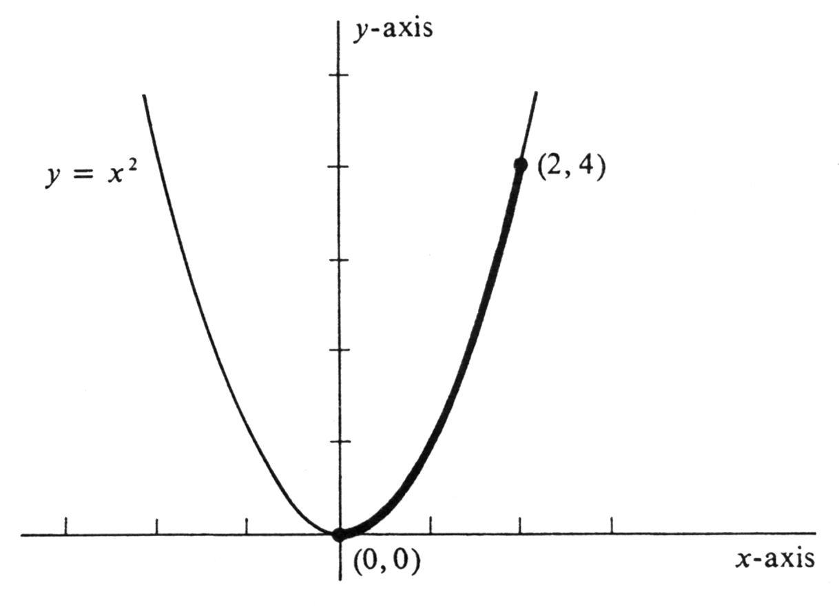
Find the arc length [math]L[/math] of the graph of the equation [math]y = x^2[/math] from the point (0, 0) to the point (2, 4). The curve is the familiar parabola shown in Figure 9. Using the result of the preceding theorem, we have

[[math]] L = \int_0^2 \sqrt{1 + \Bigl(\frac{dy}{dx}\Bigr)^2} \;dx . [[/math]]

Since [math]\frac{dy}{dx} = 2x[/math],

[[math]] L = \int_0^2 \sqrt{1 + 4x^2} \;dx . [[/math]]

This integral can be evaluated by means of the trigonometric substitution [math]x = \frac{1}{2} \tan \theta[/math], or, equivalently, [math]2x = \tan \theta[/math]. If [math]x = 0[/math], then [math] \theta = 0[/math], and, similarly, if [math]x = 2[/math], then [math] \theta = \arctan 4[/math]. For convenience we shall set [math]\arctan 4 = \theta_0[/math]. The substitution yields [math] \sqrt{1 + 4x^2} = \sqrt{1 + \tan^2 \theta} = \sec \theta[/math], and [math]dx = \frac{1}{2} \sec^2 \theta d \theta[/math]. Hence using the Change of Variable Theorem for Definite Integrals, we obtain

[[math]] \int_0^2 \sqrt{1 + 4x^2} \;dx = \frac{1}{2} \int_0^{\theta_0} \sec^3 \theta d\theta. [[/math]]

The reduction formula on page 369 gives

[[math]] \int \sec^3 \theta = \frac{\sec \theta \tan \theta}{2} + \frac{1}{2} \int \sec \theta d\theta , [[/math]]

and also on page 369 we have

[[math]] \int \sec \theta d\theta = \ln |\sec \theta + \tan \theta| + c. [[/math]]

It follows that

[[math]] \begin{eqnarray*} L = \frac{1}{2} \int_0^{\theta_0} \sec^3 \theta d\theta &=& \left[ \frac{\sec \theta \tan \theta}{4} + \frac{1}{4} \ln |\sec \theta + \tan \theta| \right]_0^{\theta_0} \\ &=& \frac{1}{4} [ \sec \theta_0 \tan \theta_0 + \ln |\sec \theta_0 + \tan \theta_0| ]. \end{eqnarray*} [[/math]]

Since [math]\theta_0 = \arctan 4[/math], we have [math]\tan \theta_0 = 4[/math] and [math]\sec \theta_0 = \sqrt{1 + \tan^2 \theta_0} = \sqrt{17}[/math]. Hence the arc length [math]L[/math] is equal to

[[math]] \begin{eqnarray*} L &=& \frac{1}{4}[\sqrt{17} \cdot 4 + \ln(\sqrt{17} + 4)] \\ &=& \sqrt{17} + \frac{1}{4} \ln(\sqrt{17} + 4) \\ &=& 4.64\;(\mathrm{approximately}). \end{eqnarray*} [[/math]]

General references

Doyle, Peter G. (2008). "Crowell and Slesnick's Calculus with Analytic Geometry" (PDF). Retrieved Oct 29, 2024.