guide:8310ca7964

[math] \newcommand{\ex}[1]{\item } \newcommand{\sx}{\item} \newcommand{\x}{\sx} \newcommand{\sxlab}[1]{} \newcommand{\xlab}{\sxlab} \newcommand{\prov}[1] {\quad #1} \newcommand{\provx}[1] {\quad \mbox{#1}} \newcommand{\intext}[1]{\quad \mbox{#1} \quad} \newcommand{\R}{\mathrm{\bf R}} \newcommand{\Q}{\mathrm{\bf Q}} \newcommand{\Z}{\mathrm{\bf Z}} \newcommand{\C}{\mathrm{\bf C}} \newcommand{\dt}{\textbf} \newcommand{\goesto}{\rightarrow} \newcommand{\ddxof}[1]{\frac{d #1}{d x}} \newcommand{\ddx}{\frac{d}{dx}} \newcommand{\ddt}{\frac{d}{dt}} \newcommand{\dydx}{\ddxof y} \newcommand{\nxder}[3]{\frac{d^{#1}{#2}}{d{#3}^{#1}}} \newcommand{\deriv}[2]{\frac{d^{#1}{#2}}{dx^{#1}}} \newcommand{\dist}{\mathrm{distance}} \newcommand{\arccot}{\mathrm{arccot\:}} \newcommand{\arccsc}{\mathrm{arccsc\:}} \newcommand{\arcsec}{\mathrm{arcsec\:}} \newcommand{\arctanh}{\mathrm{arctanh\:}} \newcommand{\arcsinh}{\mathrm{arcsinh\:}} \newcommand{\arccosh}{\mathrm{arccosh\:}} \newcommand{\sech}{\mathrm{sech\:}} \newcommand{\csch}{\mathrm{csch\:}} \newcommand{\conj}[1]{\overline{#1}} \newcommand{\mathds}{\mathbb} [/math]

Area between Curves.

Let [math]f[/math] be a function which is integrable over the interval [math][a, b][/math] and whose graph may cross the [math]x[/math]-axis a finite number of times in the interval. It was shown in Section 4 that the relation between area and the definite integral is given by the formula

[[math]] \begin{equation} \int_{a}^{b} f(x) dx = area(P^{+}) - area(P^{-}), \label{eq4.7.1} \end{equation} [[/math]]

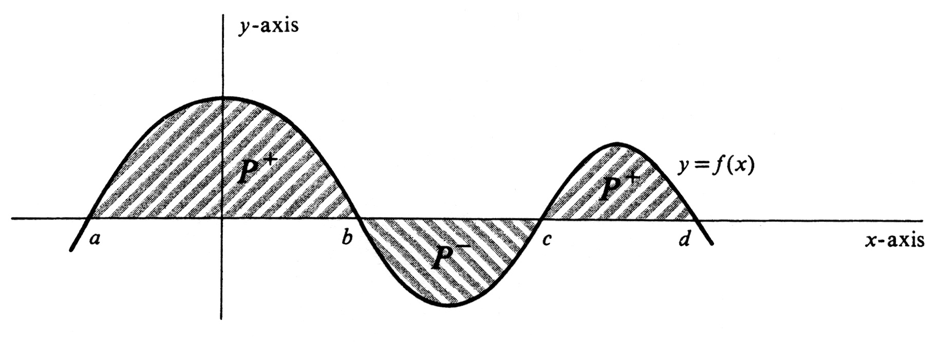
where [math]P^{+}[/math] is the set of all points [math](x,y)[/math] such that [math]a \leq x \leq b[/math] and [math]0 \leq y \leq f(x)[/math], and [math]P^{-}[/math] is the set of all points [math](x, y)[/math] such that [math]a \leq x \leq b[/math] and [math]f(x) \leq y \leq 0[/math]. If we exclude their boundaries, then either or both of the regions [math]P^{+}[/math] and [math]P^{-}[/math] may consist of several pieces. This possibility is illustrated in Figure, which shows the graph of a continuous function [math]f[/math] which crosses the [math]x[/math]-axis at the four points [math]a[/math], [math]b[/math], [math]c[/math], and [math]d[/math]. For the regions shown in the figure, we have

File:Guide c5467 scanfig4 17.png

[[math]] \begin{eqnarray*} area(P^{+}) &=& \int_{a}^{b} f(x) dx + \int_{c}^{d} f(x) dx,\\ area(P^{-}) &=& - \int_{b}^{c} f(x) dx. \end{eqnarray*} [[/math]]

Since [math]area(P^{+} \cup P^{-}) = area(P^{+}) + area(P^{-})[/math], it follows that

[[math]] area(P^{+} \cup P^{-}) = \int_{a}^{b} f(x) dx - \int_{b}^{c} f(x) dx + \int_{c}^{d} f(x) dx. [[/math]]

Suppose in this example that [math]F[/math] is an antiderivative of [math]f[/math] on the interval [math][a, d][/math]; i.e., we have [math]F'(x) = f(x)[/math] for every [math]x[/math] in [math][a, d][/math]. Then

[[math]] \begin{eqnarray*} \int_{a}^{b} f(x) dx &=& F(b) - F(a),\\ \int_{b}^{c} f(x) dx &=& F(c) - F(b), \\ \int_{c}^{d} f(x) dx &=& F(d) - F(c). \end{eqnarray*} [[/math]]

Hence the total area is given by

[[math]] \begin{eqnarray*} area(P^{+} \cup P^{-}) &=& [F(b) - F(a)] - [F(c) - F(b)] + [F(d) - F(c)] \\ &=& -F(a) + 2F(b) - 2F(c) + F(d). \end{eqnarray*} [[/math]]

In this section we shall extend (1) to compute the areas of regions with more complicated boundaries. The principal result here is the following:

Theorem

The region [math]R[/math] is illustrated in Figure(a). The only complicating feature of the proof is the fact that [math]g[/math] or [math]f[/math], or both, may take on negative values in the interval [math][a, b][/math]. If this happens [as it does in Figure(a)], we shall simply slide, or translate, the graphs of [math]g[/math] and [math]f[/math] upward so that the region between them lies above the [math]x[/math]-axis and its area is unchanged. The sliding, or translation, is shown geometrically in Figure(b), and can be accomplished anaIytically as follows. Let [math]l[/math] be a lower bound for the values of the function [math]g[/math] on the interval [math][a, b][/math]; i.e., we choose a number [math]l[/math] such that [math]l \leq g(x)[/math] for every [math]x[/math] in [math][a, b][/math]. Such a number certainly exists since [math]g[/math] is assumed to be integrable over [math][a, b][/math], and is therefore bounded on [math][a, b][/math]. In addition, if it does happen that [math]g(x) \geq 0[/math] for every [math]x[/math] in [math][a, b][/math], then we take [math]l = 0[/math]. We now define functions [math]f^{*}[/math] and [math]g^{*}[/math] by

[[math]] \begin{eqnarray*} f^{*}(x) &=& f(x) + |l|, \\ g^{*}(x) &=& g(x) + |l|. \end{eqnarray*} [[/math]]

Their graphs and the region between them, which is denoted by [math]R^{*}[/math], is shown in Figure(b). It is obvious that

[[math]] area(R) = area(R^*). [[/math]]

Let [math]P[/math] be the set of points bounded by the graph of [math]g^{*}[/math], the [math]x[/math]-axis, and the lines [math]x = a[/math] and [math]x = b[/math]. By the integral formula for area, we know that

[[math]] \begin{eqnarray*} area(P \cup R^{*}) &=& \int_{a}^{b} f^{*}(x) dx,\\ area(P) &=& \int_{a}^{b} g^{*}(x) dx. \end{eqnarray*} [[/math]]

Since [math]area(R^{*}) = area(P \cup R^{*}) - area(P)[/math], we obtain

[[math]] \begin{eqnarray*} area(R) &=& area(R^{*}) = \int_{a}^{b} f^{*}(x) dx - \int_{a}^{b} g^{*}(x) dx \\ &=& \int_{a}^{b} [f^{*}(x) - g^{*}(x)]dx. \end{eqnarray*} [[/math]]

However,

[[math]] \begin{eqnarray*} f^{*}(x) - g^{*}(x) &=& [f(x) + |l| ] - [g(x) + |l| ] \\ &=& f(x) - g(x). \end{eqnarray*} [[/math]]

Hence

[[math]] area(R) = \int_{a}^{b} [f(x) - g(x)] dx, [[/math]]

and the proof is complete.

Show Proof

{{{4}}}

■

It should be remarked that, rigorously speaking, the above proof omits some logical details. These occur in our use of the function area. To begin with, we have not in this book attempted to give a mathematical definition of the area of a set, although we have shown that if area does exist and satisfies certain simple properties, then the integral formula (1) is valid. Moreover, in the preceding paragraph we have tacitly assumed some of the properties of area which are obvious to the intuition, but logically would require proof. For example, we assumed that area is invariant under translation when we asserted that [math]area(R)= area(R^{*})[/math]. In the same way, our statement that [math]area(R^{*}) = area(P \cup R^{*}) - area(P)[/math] [see Figure(b)] was based solely on geometric intuition. There is nothing wrong with omitting these details, but it is important that a careful reader realize that the omissions are there. Example

Compute the area of the region [math]R[/math] bounded by the graphs of the functions [math]f(x) = 2x - 1[/math] and [math]g(x) = - (2x - 1)^2[/math]. and the lines [math]x = 1[/math] and [math]x= 2[/math]. Since

[[math]] \begin{eqnarray*} g(x) \leq 0, && \;\;\;\mbox{for every}\; x, \\ f(x) \geq 0, &&\;\;\;\mbox{if}\; 1 \leq x \leq 2, \end{eqnarray*} [[/math]]

it follows that [math]g(x) \leq f(x)[/math] on the interval [1, 2]. Both functions are continuous and hence integrable, and so (7.1) is applicable. We obtain

[[math]] area(R) = \int_{1}^{2} [f(x) - g(x)] dx. [[/math]]

Since [math]f(x)-g(x) = (2x-1) + (2x-1)^2 = 4x^2 - 2x[/math], the answer is

[[math]] \begin{eqnarray*} area(R) &=& \int_{1}^{2} (4x^2 - 2x) dx = (\frac{4}{3}x^3 - x^2) \Big|_{1}^{2}\\ &=& (\frac{32}{3} - 4) - (\frac{4}{3} - 1) = \frac{19}{3}. \end{eqnarray*} [[/math]]

\medskip Example

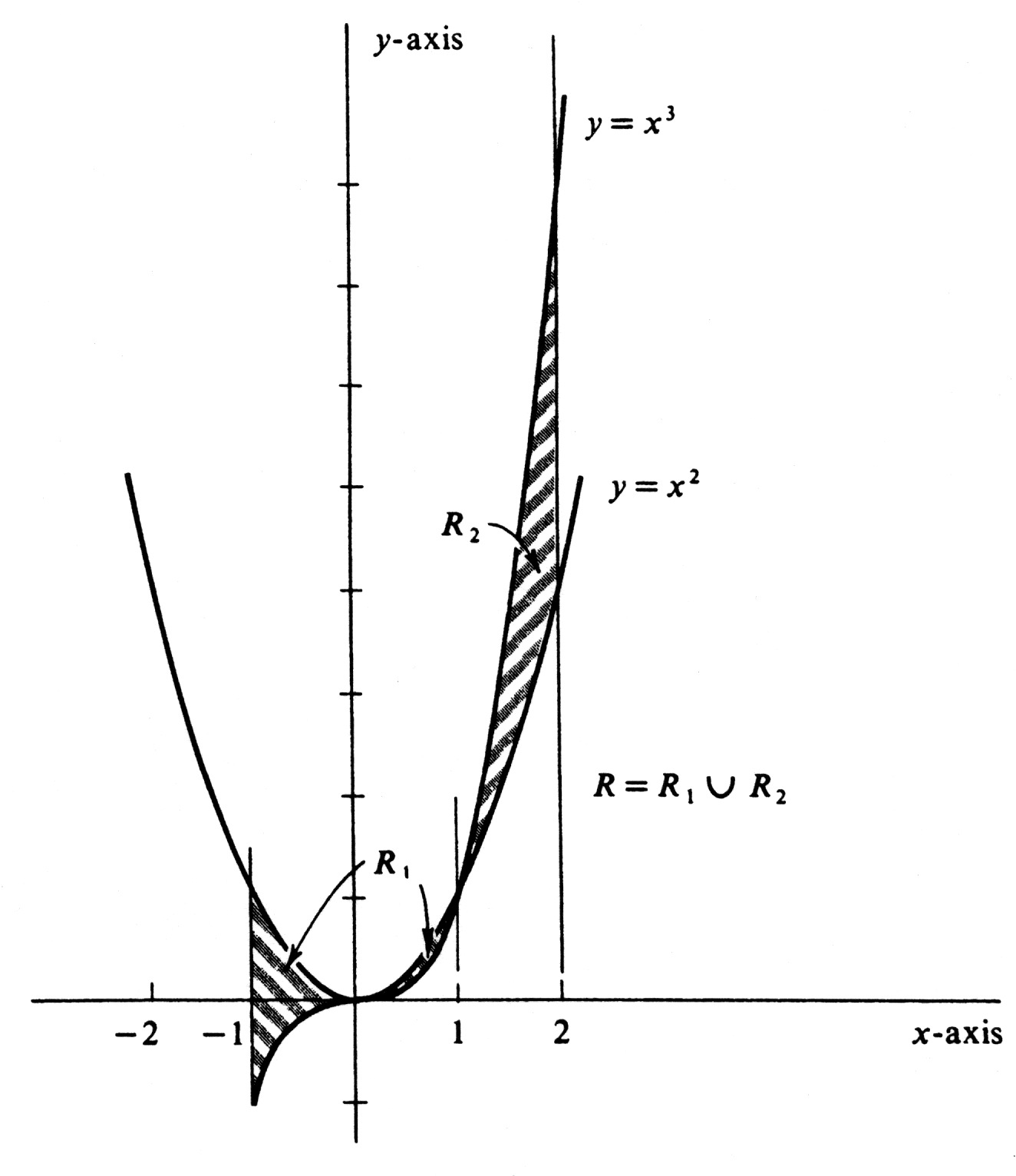
Find the area of the region [math]R[/math] lying between the lines [math]x = - 1[/math] and [math]x = 2[/math] and between the curves [math]y = x^2[/math] and [math]y = x^3[/math]. We first sketch the lines and curves in question and indicate the region [math]R[/math] by shading (see Figure). Observe that

[[math]] \begin{eqnarray*} x^3 \leq x^2, &&\;\;\;\mbox{if}\; - 1 \leq x \leq 1,\\ x^2 \leq x^3, &&\;\;\;\mbox{if}\; 1 \leq x \leq 2. \end{eqnarray*} [[/math]]

File:Guide c5467 scanfig4 19.png

Writing [math]R[/math] as the union of regions [math]R_1[/math] and [math]R_2[/math], as is done in the figure, we have, by (7.1),

[[math]] \begin{eqnarray*} area(R_1) &=& \int_{-1}^{1} (x^2 - x^3) dx, \\ area(R_2) &=& \int_{1}^{2} (x^3 - x^2) dx. \end{eqnarray*} [[/math]]

Hence

[[math]] \begin{eqnarray*} area(R) &=& area(R_1) + area(R_2)\\ &=& \int_{-1}^{1} (x^2 - x^3) dx + \int_{1}^{2} (x^3 - x^2) dx. \end{eqnarray*} [[/math]]

The function [math]F(x) =\frac{x^3}{3} - \frac{x^4}{4}[/math] is clearly an indefinite integral of [math]x^2 - x^3[/math]. Thus

[[math]] \begin{eqnarray*} \int_{-1}^{1} (x^2 - x^3)dx &=& F(x) \Big|_{-1}^{1} = F(1) - F( - 1),\\ \int_{1}^{2} (x^3 - x^2) dx &=& - \int_{1}^{2} (x^2 - x^3)dx\\ &=& -F(x) \Big|_{1}^{2} = - F(2) + F(1). \end{eqnarray*} [[/math]]

Finally, therefore,

[[math]] \begin{eqnarray*} area(R) &=& F(1) - F( - 1) - F(2) + F(1)\\ &=& \frac{1}{12} + \frac{7}{12} + \frac{4}{3} + \frac{1}{12} = \frac{25}{12}. \end{eqnarray*} [[/math]]

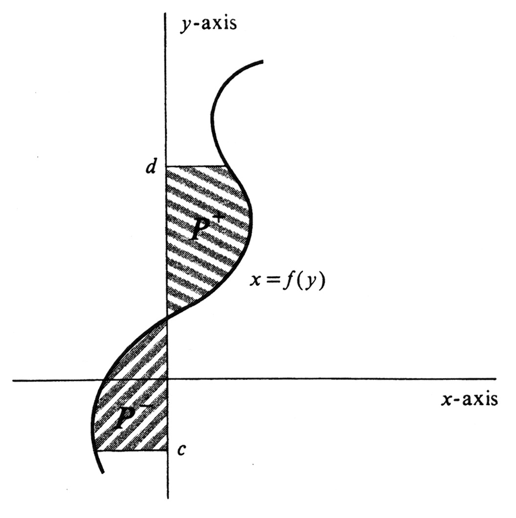
\medskip Because of symmetry, each of the integral formulas for area which we have developed has an obvious counterpart for functions of [math]y[/math]. For example, if [math]f[/math] is the function of [math]y[/math] whose graph is drawn in Figure, then

[[math]] \int_{c}^{d} f(y) dy = area(P^{+}) - area(P^{-}), [[/math]]

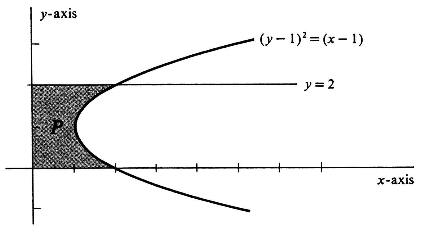
where [math]P^{+}[/math] and [math]P^{-}[/math] are the regions indicated in the figure. Sometimes a curve in the [math]xy[/math]-plane can be defined as the graph of a function of [math]y[/math] and not as a function of [math]x[/math]. An example is the parabola defined by the equation [math](y -1)^2 = x - 1[/math] and illustrated in Figure. Although this equation cannot be solved uniquely for [math]y[/math] in terms of [math]x[/math], it is easy to do the opposite. We get

[[math]] x = (y -1)^2 + 1 = y^2 - 2y + 2, [[/math]]

and so the curve is the graph of the function [math]f[/math] defined by [math]f(y) = y^2 - 2y + 2[/math]. The area of the region [math]P[/math] bounded by the parabola, the two coordinate axes, and the horizontal line [math]y = 2[/math] is given by

[[math]] \begin{eqnarray*} area(P) &=& \int_{0}^{2} f(y)dy = \int_{0}^{2} (y^2 - 2y + 2) dy \\ &=& \Bigl( \frac{y^3}{3} - y^2 + 2y \Bigr) \Big|_{0}^{2} = \frac{8}{3}. \end{eqnarray*} [[/math]]

File:Guide c5467 scanfig4 20.png

File:Guide c5467 scanfig4 21.png

Example

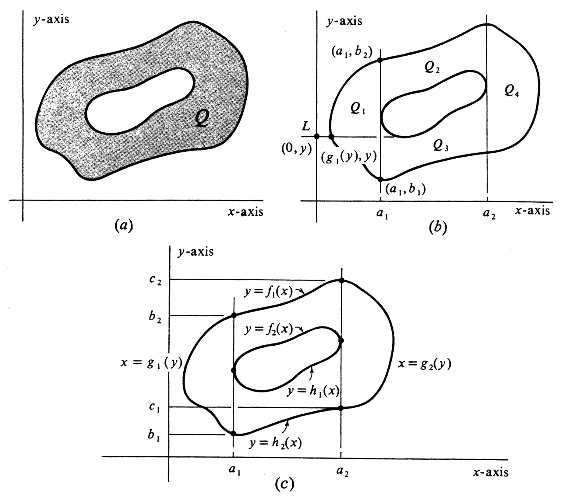
Express the area of the shaded region [math]Q[/math] in Figure(a) as a sum of definite integrals. There are many different ways to do this. We shall begin by subdividing [math]Q[/math] into four subregions [math]Q_1[/math], [math]Q_2[/math], [math]Q_3[/math], and [math]Q_4[/math] using the two vertical lines [math]x = a_1[/math], and [math]x = a_2[/math] as shown in Figure(b). Consider for a moment the region [math]Q_1[/math] alone. Every horizontal line [math]L[/math] which intersects [math]Q_1[/math] cuts its boundary in at most two points. Suppose that [math]L[/math] crosses the [math]y[/math]-axis at the point [math](0, y)[/math]. Moving along [math]L[/math] from left to right, we denote the [math]x[/math]-coordinate of the first point encountered on the boundary of [math]Q_1[/math], by [math]g_{1}(y)[/math]. In this way a function [math]g_{1}[/math] is defined whose graph forms the “western boundary” of [math]Q_{1}[/math]. In fact, [math]Q_1[/math] is the region between [math]y = b_1[/math] and [math]y = b_2[/math] [see Figure(b)] and also between the curves [math]x = g_{1}(y)[/math] and [math]x = a_1[/math]. By the counterpart of (7.1) for functions of [math]y[/math], we therefore obtain

[[math]] area(Q_1) = \int_{b_1}^{b_2} [a_1 - g_1(y)] dy. [[/math]]

File:Guide c5467 scanfig4 22.png

Turning next to the region [math]Q_2[/math], we see that the “northern boundary” is the graph of a function [math]f_1[/math], and the “southern boundary” is the graph of a function [math]f_2[/math]. These functions are indicated in Figure(c). Hence

[[math]] area( Q_2) = \int_{a_1}^{a_2} [f_{1}(x) - f_{2}(x)]dx. [[/math]]

Similarly, we have

[[math]] area(Q_3) = \int_{a_1}^{a_2} [h_{1}(x) - h_{2}(x)] dx, [[/math]]

and also

[[math]] area(Q_4) = \int_{c_1}^{c_2} [g_{2}(y) - a_{2}]dy. [[/math]]

Since [math]area(Q) = area(Q_1) + area(Q_2) + area(Q_3) + area(Q_4)[/math], we therefore obtain finally

[[math]] \begin{eqnarray*} area(Q) = && \int_{b_1}^{b_2} [a_{1} - g_{1}(y)] dy + \int_{a_1}^{a_2} [f_{1}(x) - f_{2}(x)] dx \\ &&+ \int_{a_1}^{a_2} [h_{1}(x) - h_{2}(x)] dx + \int_{c_1}^{c_2} [g_{2}(y) - a_{2}] dy. \end{eqnarray*} [[/math]]

\end{exercise}

General references

Doyle, Peter G. (2008). "Crowell and Slesnick's Calculus with Analytic Geometry" (PDF). Retrieved Oct 29, 2024.