guide:A8103d1e65

[math] \newcommand{\ex}[1]{\item } \newcommand{\sx}{\item} \newcommand{\x}{\sx} \newcommand{\sxlab}[1]{} \newcommand{\xlab}{\sxlab} \newcommand{\prov}[1] {\quad #1} \newcommand{\provx}[1] {\quad \mbox{#1}} \newcommand{\intext}[1]{\quad \mbox{#1} \quad} \newcommand{\R}{\mathrm{\bf R}} \newcommand{\Q}{\mathrm{\bf Q}} \newcommand{\Z}{\mathrm{\bf Z}} \newcommand{\C}{\mathrm{\bf C}} \newcommand{\dt}{\textbf} \newcommand{\goesto}{\rightarrow} \newcommand{\ddxof}[1]{\frac{d #1}{d x}} \newcommand{\ddx}{\frac{d}{dx}} \newcommand{\ddt}{\frac{d}{dt}} \newcommand{\dydx}{\ddxof y} \newcommand{\nxder}[3]{\frac{d^{#1}{#2}}{d{#3}^{#1}}} \newcommand{\deriv}[2]{\frac{d^{#1}{#2}}{dx^{#1}}} \newcommand{\dist}{\mathrm{distance}} \newcommand{\arccot}{\mathrm{arccot\:}} \newcommand{\arccsc}{\mathrm{arccsc\:}} \newcommand{\arcsec}{\mathrm{arcsec\:}} \newcommand{\arctanh}{\mathrm{arctanh\:}} \newcommand{\arcsinh}{\mathrm{arcsinh\:}} \newcommand{\arccosh}{\mathrm{arccosh\:}} \newcommand{\sech}{\mathrm{sech\:}} \newcommand{\csch}{\mathrm{csch\:}} \newcommand{\conj}[1]{\overline{#1}} \newcommand{\mathds}{\mathbb} [/math]

The Derivative.

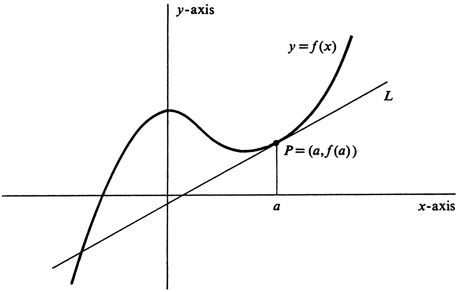
The concept of the line tangent to a curve at a point is an important one in geometry. However, it is not so simple an idea as it may first appear. Consider the graph of a function [math]f[/math] and a point [math]P = (a, f(a))[/math] on the graph, as illustrated in Figure.

File:Guide c5467 scanfig1 33.png

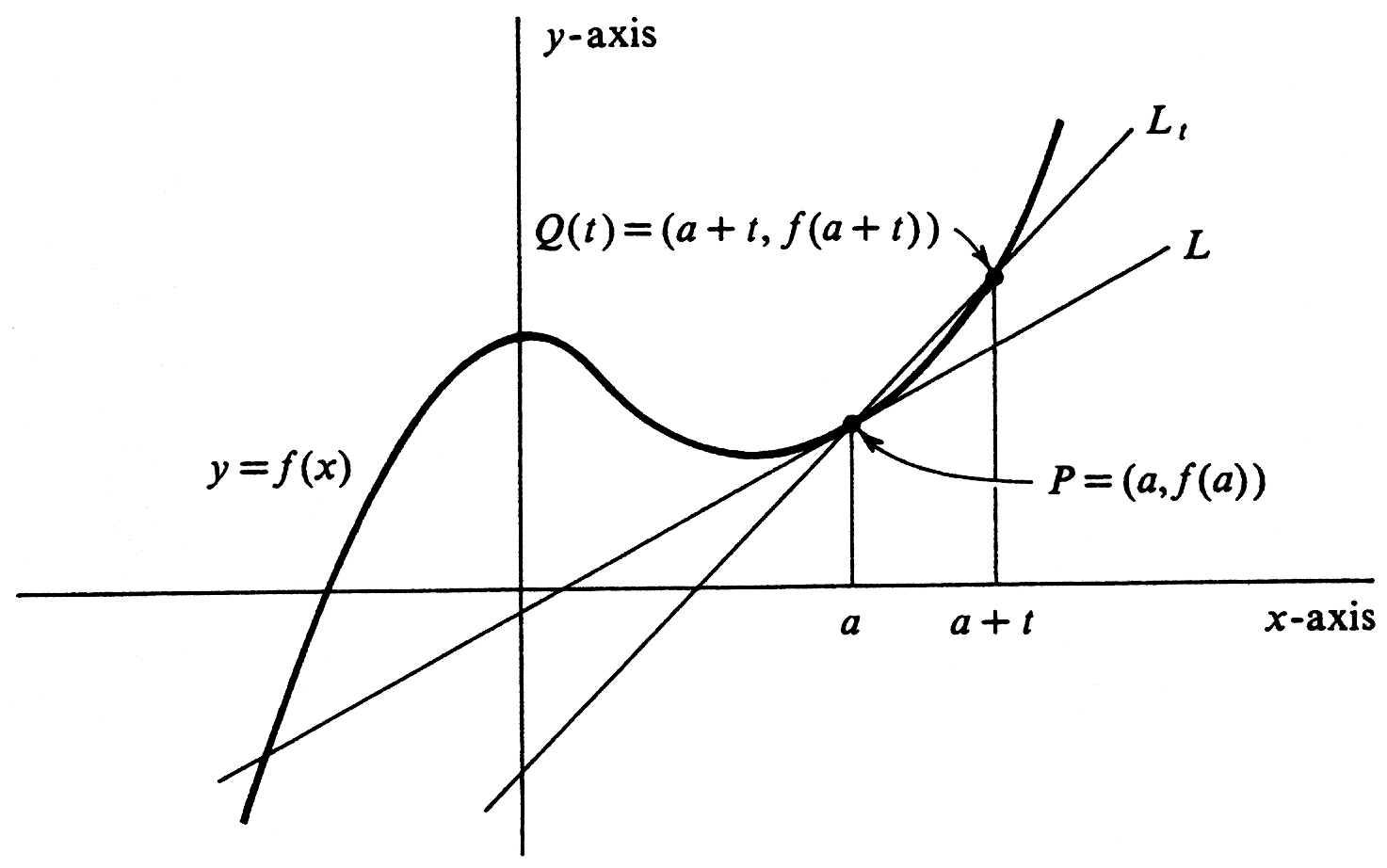
Many people who would have little difficulty drawing the line tangent to the graph at [math]P[/math] would not find it easy to give an accurate definition of the tangent line. For example, to say that the tangent line at [math]P[/math] is the line which cuts the graph at the single point [math]P[/math], although true for some curves, is obviously not correct in general (in particular, see Figure. We shall show that the problem of defining the tangent line to the graph of [math]f[/math] at [math]P[/math] can be expressed in purely analytic terms involving the function [math]f[/math]. In fact, the problem leads directly to the definition of the derivative of a function, the central idea in differential calculus. Let [math]t[/math] be an arbitrary nonzero real number, and consider the point [math]Q(t) = (a + t, f(a + t))[/math], which, together with [math]P = (a, f(a))[/math], lies on the graph of [math]f[/math] (see Figure).

File:Guide c5467 scanfig1 34.png

The slope of the secant line [math]L_t[/math] containing [math]P[/math] and [math]Q(t)[/math] is equal to

[[math]] \begin{equation} m(P, Q(t)) = \frac{f(a + t) - f(a)}{t} . \label{eq1.6.1} \end{equation} [[/math]]

If [math]t[/math] is small in absolute value, then [math]L_t[/math] is an approximation to what we shall define to be the tangent line. The smaller the value of [math]|t|[/math], the better the approximation will be. In some sense, therefore, we would like to define the tangent line [math]L[/math] to be the limit, as [math]t[/math] approaches zero, of the lines [math]L_t[/math]. We can do this, for although we have not defined a limit of lines, we have defined limits for functions, and hence we can express the limit of the slope of [math]L_t[/math]. According to equation 1.6.1, it is given by

[[math]] \begin{equation} \lim_{t \rightarrow 0}{m(P,Q(t))} = \lim_{t \rightarrow 0}{\frac{f(a + t) - f(a)}{t}} . \label{eq1.6.2} \end{equation} [[/math]]

We shall define the tangent line to the graph of [math]f[/math] at [math]P[/math] to be the line through [math]P[/math] having this limit as its slope, provided the limit exists. Leaving the geometric interpretation aside for the moment, we observe that the value of the limit in depends only on the function [math]f[/math] and on the number [math]a[/math]. Hence we give the following definitions: An arbitrary real-valued function [math]f[/math] of a real variable is differentiable at a number [math]a[/math] in its domain if

[[math]] \lim_{t \rightarrow 0}{\frac{f(a + t) - f(a)}{t}} [[/math]]

exists (i.e., is finite). The derivative of [math]f[/math] at [math]a[/math], denoted [math]f'(a)[/math], is this limit. Thus

[[math]] f'(a) = \lim_{t \rightarrow 0}{\frac{f(a + t) - f(a)}{t}} . [[/math]]

If [math]f[/math] is differentiable at every number in its domain, it is simply called a differentiable function. Thus the slope of the line tangent to the graph of [math]f[/math] at the point [math](a, f(a))[/math] is equal to the derivative [math]f'(a)[/math]. It follows that an arbitrary point [math](x, y)[/math] lies on this line if and only if

[[math]] y - f(a) = f'(a)(x - a) , [[/math]]

and we therefore obtain the following equation of the tangent line:

[[math]] y = f(a) + f'(a)(x - a) . [[/math]]

Note that the only variables that appear in this equation are [math]x[/math] and [math]y[/math], and these occur with exponent 1. The equation therefore defines [math]y[/math] as a linear function of [math]x[/math].

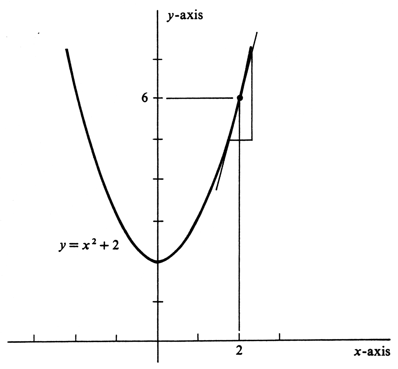
Example

Find the derivative of the function [math]f(x) = x^2 + 2[/math] at [math]x = 2[/math], and write an equation of the line tangent to the graph of [math]f[/math] at the point [math](2, 6)[/math]. As we have seen above, the slope of the tangent line is the derivative [math]f'(2)[/math], and

[[math]] f'(2) = \lim_{t \rightarrow 0} {\frac{f(2 + t) - f(2)}{t}} . [[/math]]

We have [math]f(2) = 6[/math], and [math]f(2 + t) = (2 + t)^2 + 2 = t^2 + 4t + 6 .[/math] Hence

[[math]] \frac{f(2 + t) - f(2)}{t} = \frac{t^2 + 4t}{t} = t + 4, \;\;\;\mbox{if} t \neq 0. [[/math]]

So

[[math]] f'(2) = \lim_{t \rightarrow 0} (t + 4) = 4 . [[/math]]

The tangent line passes through (2, 6) and has slope 4. Hence [math](x, y)[/math] lies on the tangent if

[[math]] \frac{y - 6}{x - 2} = 4, \;\;\; x \neq 2 , [[/math]]

and we therefore obtain

[[math]] y - 6 = 4(x - 2) \;\;\; \mbox{or}\;\;\; 4x - y - 2 = 0 , [[/math]]

as an equation of the line.

Example

Consider the function [math]g[/math] defined by

[[math]] g(x)= \frac{1}{x + 2} , \;\;\; x \neq -2 . [[/math]]

Compute the derivative [math]g'(3)[/math]. By definition,

[[math]] g'(3) = \lim_{x \rightarrow 0} {\frac{g(3 + t) - g(3)}{t}} . [[/math]]

We have [math]g(3) = \frac{1}{5}[/math], and [math]g(3 + t) = \frac{1}{t + 5}[/math] .

[[math]] \begin{eqnarray*} \frac{g(3 + t) - g(3)}{t} &=& \frac{1}{t} \Bigl( \frac{1}{t + 5} - \frac{1}{5} \Bigr)\\ &=& \frac{5 - (t + 5)}{5t (t + 5)} \\ &=& - \frac{t}{5t (t + 5)} \\ &=& - \frac{1}{5 (t + 5)}, \provx{if $t \neq 0$} . \end{eqnarray*} [[/math]]

We conclude that

[[math]] g'(3) = \lim_{t \rightarrow 0} \Bigl(- \frac{1}{5(t + 5)} \Bigr) = - \frac{1}{25} . [[/math]]

Example

Find [math]F'(a)[/math], where [math]a \gt 0[/math] and [math]F[/math] is the function

[[math]] F(x) = \frac{1}{x^{\frac{1}{2}}}, \;\;\; 0 \lt x \lt \infty , [[/math]]

and write an equation of the line tangent to the graph of [math]F[/math] at the point (4, [math]\frac{1}{2}[/math]). By the definition of the derivative,

[[math]] F'(a) = \lim_{x \rightarrow 0} { \frac{F(a + t) - F(a)}{t} } . [[/math]]

In this case,

[[math]] \frac{F(a + t) - F(a)}{t} = \frac{1}{t} \Bigl( \frac{1}{\sqrt{a + t}} - \frac{1}{\sqrt a} \Bigr) . [[/math]]

The problem in computing any derivative from the definition is always the same. We set up the fraction [math]\frac{F(a + t) - F(a)}{t}[/math] and then compute the limit. To begin with, we are faced with a fraction both the numerator and denominator of which approach zero. The limit we seek is the relative rate at which numerator and denominator go to zero. With most examples it is not possible to tell from a cursory glance just what that relative rate is. So we experiment, performing various algebraic manipulations that hopefully will finally change the fraction into a form from which we can tell what the limit is. In the present example the following manipulation will do the trick:

[[math]] \begin{eqnarray*} \frac{1}{t} \Bigl( \frac{1}{\sqrt{a + t}} - \frac{1}{\sqrt a} \Bigr) &=& {\frac{1}{t}} {\frac{\sqrt{a} - \sqrt(a + t)}{\sqrt{a} \sqrt{a + t}} } {\frac{\sqrt{a} + \sqrt{a + t}}{\sqrt{a} + \sqrt{a + t}} } \\ &=& {\frac{1}{t}} {\frac{a - (a + t)}{\sqrt{a} \sqrt{a + t} (\sqrt{a} + \sqrt{a + t})} }\\ &=& \frac {-1} {\sqrt{a^2 + at} (\sqrt{a} + \sqrt{a + t} ) }, \provx{if $t \neq 0$}. \end{eqnarray*} [[/math]]

It is now possible to see what happens as [math]t \rightarrow 0[/math].

[[math]] F'(a) = \lim_{x \rightarrow 0} { \frac{-1}{ \sqrt{a^2 + at} (\sqrt{a} + \sqrt{a + t}) } } = \frac{-1}{2a \sqrt{a}} = - \frac{1}{2a^{3/2}} . [[/math]]

Our principal interpretation of the derivative [math]F'(a)[/math] is that it is the slope of the line tangent to the graph of [math]F[/math] at the point [math](a, F(a))[/math]. For this particular function [math]F[/math], an equation of the tangent line at [math](4, \frac{1}{2})[/math] is therefore found by writing

[[math]] \frac{y - \frac{1}{2}}{x - 4} = F'(4) = -\frac{1}{2 \cdot 4^{\frac{3}{2}}} = -\frac{1}{16} . [[/math]]

Hence an equation of the tangent is

[[math]] y - \frac{1}{2} = - {\frac{1}{16}} (x - 4). [[/math]]

The notation [math]f'(a)[/math] for the derivative suggests that we regard [math]f'[/math] as a new function whose value at [math]a[/math] is the number [math]f'(a)[/math]. The domain of [math]f'[/math] is the set of all real numbers [math]a[/math] for which [math]\lim_{t \rightarrow 0} \frac{f(a + t) - f(a)}{t}[/math] exists. With this point of view, it is natural to think of the derivative evaluated not only at an arbitrary, but fixed, number [math]a[/math] but also at a variable [math]x[/math]. In so doing, we are admitting the same dual interpretations that were discussed in Section \secref{1.3}. That is, we can interpret [math]f'(x)[/math] either as the value of the function [math]f'[/math] at the number [math]x[/math], whence

[[math]] f'(x) = \lim_{t \rightarrow 0} \frac{f(x + t) - f(x)}{t}, [[/math]]

or as the composition of the variable [math]x[/math] with the function [math]f'[/math].

Example

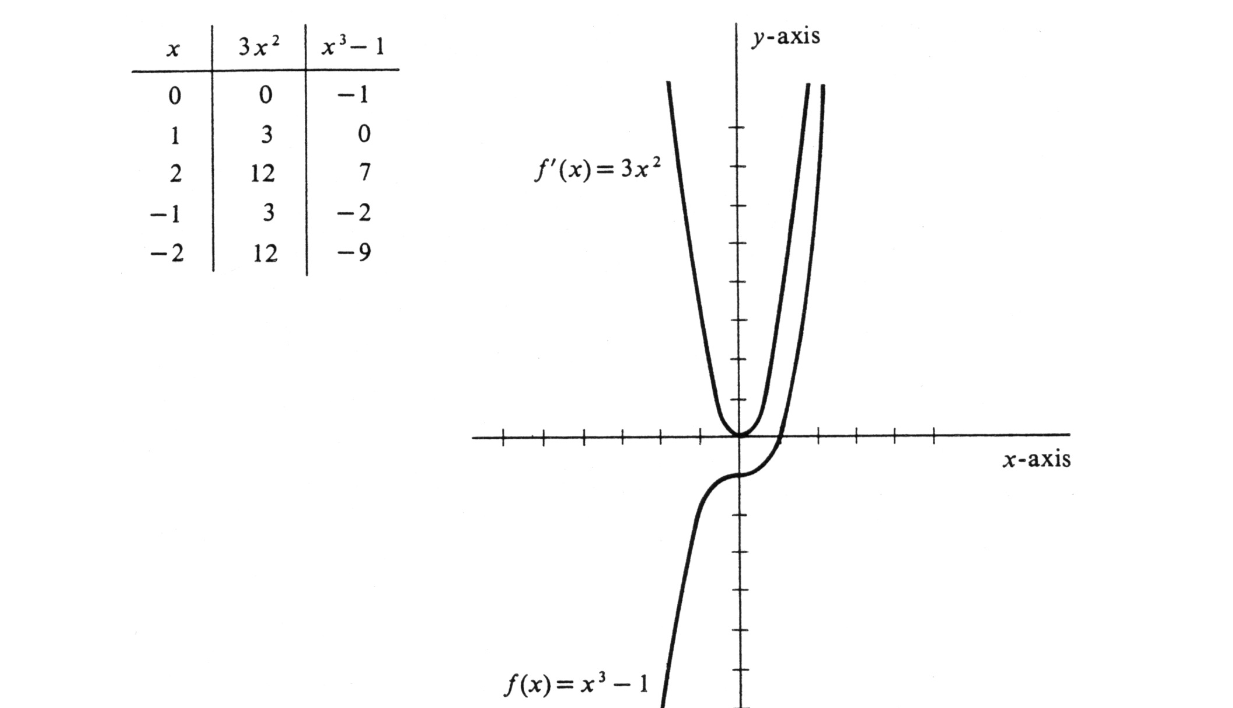
If [math]f(x) = x^3 - 1[/math], plot the graph of the derived function [math]f'[/math]. For any real number [math]x[/math],

[[math]] f'(x) = \lim_{t \rightarrow 0} \frac {f(x + t) - f(x)}{t} . [[/math]]

We have

[[math]] \begin{eqnarray*} f(x + t) - f(x) &=& ((x + t)^3 - 1) - (x^3 - 1) \\ &=& 3x^2t + 3xt^2 + t^3 , \end{eqnarray*} [[/math]]

and so

[[math]] \frac {f(x + t) - f(x)}{t} = 3x^2 + 3xt + t^2, \provx{if $t \neq 0$}. [[/math]]

Consequently,

[[math]] f'(x) = \lim_{t \rightarrow 0} (3x^2 + 3xt + t^2) = 3x^2 . [[/math]]

The graph of the function [math]f'(x) = 3x^2[/math] is the parabola shown in Figure,

File:Guide c5467 scanfig1 35.png

on which the graph of the original function [math]f(x) = x^3 - 1[/math] has also been drawn.

It is not surprising that there are several common notations for the derivative of a function. One strong tradition reflects the basic fact that the derivative is the limit of a ratio by writing it as a ratio. Thus

[[math]] \frac{df}{dx} = f' . [[/math]]

This way of writing the derivative is called the differential notation. Using it, we denote the derivative of [math]f[/math] at [math]a[/math] by

[[math]] \frac{df}{dx} (a) = f'(a) . [[/math]]

Example

Let [math]f(x) = x^3 - 1[/math]. It was shown in Example that [math]f'(x) = 3x^2[/math]. Each of the following equations is an example of acceptable notation.

[[math]] \begin{eqnarray*} \frac{df}{dx} (2) &=& 3 \cdot 2^2 = 12 , \\ \frac{df}{dx} (a) &=& 3a^2 , \\ \frac{df}{dx} &=& 3x^2 , \\ \frac{d}{dx} (x^3 - 1) &=& 3x^2 . \end{eqnarray*} [[/math]]

One could also write [math]\frac{df}{dx} (x) = f'(x) = 3x^2[/math]. There is no need for it, however, since [math]f'(x)[/math] becomes identified with [math]f'[/math] when it is regarded as the composition of the independent variable [math]x[/math] with the function [math]f'[/math].

It should be emphasized that although the notation [math]\frac{df}{dx}[/math] suggests a ratio, the derivative as we have defined it is not a ratio---even though it is the limit of one. [math]\frac{df}{dx}[/math] is simply an abbreviation of [math]f'[/math]. There are a few variations on the two notations that we have given for the derivative which we shall also use frequently. If [math]y = f(x)[/math], we may write any one of

[[math]] y' = \frac{dy}{dx} = f' = \frac{df}{dx} [[/math]]

for the derivative. Similarly, for the derivative at a real number [math]a[/math], we have

[[math]] y'(a) = {\frac{dy}{dx}} (a) = f'(a) = {\frac{df}{dx}} (a) . [[/math]]

Still other notations for the derivative, which we shall seldom use, but which the reader may encounter in other books are

[[math]] Df = D_{x}f = Dy = D_{x}y = \dot{y} , [[/math]]

where it is assumed that [math]y = f(x)[/math]. Example

It follows from the computation in Example that if [math]F(x) = x^{-1/2}[/math], [math]x \gt 0[/math], then the derivative is given by [math]F'(x) = -\frac{1}{2} x^{-3/2}[/math]. If we write [math]y = x^{-1/2}, x \gt 0[/math], the derivative is also written

[[math]] y' = \frac{dy}{dx} = - \frac{1}{2 x^{3/2}} . [[/math]]

The value of the derivative at 4 is

[[math]] y'(4) = {\frac{dy}{dx}} (4) = - \frac{1}{2 \cdot 4^{3/2}} = - \frac{1}{16} . [[/math]]

The slope of a straight line is the ratio of a change in [math]y[/math] to a change in [math]x[/math]. It therefore measures the rate of change of [math]y[/math] per unit change in [math]x[/math] for the ordered pairs [math](x, y)[/math] that make up the line. Consider the two lines defined by [math]y = 10x - 3[/math] and [math]y = x - 3[/math] respectively. The rate of change of [math]y[/math] to [math]x[/math] is [math]10[/math] for the first and 1 for the second. For a function whose graph is not a straight line, however, the concept of the rate of change of [math]y[/math], or [math]f(x)[/math], with respect to [math]x[/math] is more profound. There is the problem that the change in functional values [math]f(x)[/math] per unit change in [math]x[/math] will not be constant along the graph. More basic, however, is the question of the precise meaning or definition of the rate of change. The answer is provided by the derivative. Since [math]f'(a)[/math] is the slope of the line tangent to the graph of [math]f[/math] at the point [math](a, f(a))[/math], it measures the rate of change of [math]f(x)[/math] with respect to [math]x[/math] at that point. In Example we showed that if [math]f(x) = x^2 + 2[/math], then [math]f'(2) = 4[/math]. We interpret the number 4 not only as the slope of the line tangent to the graph of [math]f[/math] at [math](2, 6)[/math] but also as the rate of change of [math]f(x)[/math] with respect to [math]x[/math] there. From the picture of the graph in Figure

File:Guide c5467 scanfig1 36.png

it is apparent that at [math](2, 6)[/math] a small change in [math]x[/math] produces a corresponding change four times as great in [math]f(x)[/math]. In Section \secref{1.4} the idea of limit was introduced by examples and by exploiting the reader's intuitive understanding of continuity and continuous curves. We then gave a formal definition and proceeded in terms of it to go back and define continuity precisely. We shall do an analogous thing here and now define the slope of the graph of [math]f[/math] at the point [math](a, f(a))[/math], or more simply the slope of the curve [math]y = f(x)[/math] at [math](a,f(a))[/math], to be the derivative [math]f'(a)[/math]. We conclude this section with the theorem

Proposition

If a function [math]f[/math] is differentiable at [math]a[/math], then it is continuous there.

Show Proof

The hypothesis that

[[math]] \lim_{t \rightarrow 0} {\frac{f(a + t) - f(a)}{t}} [[/math]]

exists implies tacitly that [math]a[/math] is in the domain of [math]f[/math]. If a quotient approaches a finite limit as the denominator approaches zero, then the numerator must also approach zero. This fact is a consequence of the theorem that the limit of a product is the product of the limits [see part (iii) of Theorem]. In this case, we have

[[math]] \begin{eqnarray*} \lim_{t \rightarrow 0} [f(a + t) - f(a)] &=& \lim_{t \rightarrow 0} \Bigl[ {\frac{f(a + t) - f(a)}{t}} \cdot t \Bigr] \\ &=& \lim_{t \rightarrow 0} \Bigl[ \frac {f(a + t) - f(a)}{t} \Bigr] \cdot \lim_{t \rightarrow 0} t \\ &=& f'(a) \cdot 0 = 0 . \end{eqnarray*} [[/math]]

The equation [math]\lim_{t \rightarrow 0} {[f(a + t) - f(a)]} = 0[/math] is equivalent to

[[math]] \begin{equation} \lim_{t \rightarrow 0} f(a + t) = f(a) . \label{eq1.6.3} \end{equation} [[/math]]

If we set [math]x = a + t[/math], then [math]x[/math] approaches [math]a[/math] as [math]t[/math] approaches 0, and conversely. So becomes

[[math]] \lim_{x \rightarrow a} f(x) = f(a) , [[/math]]

and the proof is complete.

■

General references

Doyle, Peter G. (2008). "Crowell and Slesnick's Calculus with Analytic Geometry" (PDF). Retrieved Oct 29, 2024.