guide:27efc1ff17

[math] \newcommand{\ex}[1]{\item } \newcommand{\sx}{\item} \newcommand{\x}{\sx} \newcommand{\sxlab}[1]{} \newcommand{\xlab}{\sxlab} \newcommand{\prov}[1] {\quad #1} \newcommand{\provx}[1] {\quad \mbox{#1}} \newcommand{\intext}[1]{\quad \mbox{#1} \quad} \newcommand{\R}{\mathrm{\bf R}} \newcommand{\Q}{\mathrm{\bf Q}} \newcommand{\Z}{\mathrm{\bf Z}} \newcommand{\C}{\mathrm{\bf C}} \newcommand{\dt}{\textbf} \newcommand{\goesto}{\rightarrow} \newcommand{\ddxof}[1]{\frac{d #1}{d x}} \newcommand{\ddx}{\frac{d}{dx}} \newcommand{\ddt}{\frac{d}{dt}} \newcommand{\dydx}{\ddxof y} \newcommand{\nxder}[3]{\frac{d^{#1}{#2}}{d{#3}^{#1}}} \newcommand{\deriv}[2]{\frac{d^{#1}{#2}}{dx^{#1}}} \newcommand{\dist}{\mathrm{distance}} \newcommand{\arccot}{\mathrm{arccot\:}} \newcommand{\arccsc}{\mathrm{arccsc\:}} \newcommand{\arcsec}{\mathrm{arcsec\:}} \newcommand{\arctanh}{\mathrm{arctanh\:}} \newcommand{\arcsinh}{\mathrm{arcsinh\:}} \newcommand{\arccosh}{\mathrm{arccosh\:}} \newcommand{\sech}{\mathrm{sech\:}} \newcommand{\csch}{\mathrm{csch\:}} \newcommand{\conj}[1]{\overline{#1}} \newcommand{\mathds}{\mathbb} [/math]

Two additional methods of integration by numerical approximations, which we shall describe in this section, are the Midpoint Rule and Simpson's Rule. In the Midpoint Rule the approximation to the integral [math]\int_a^b f[/math] is a Riemann sum [math]\sum_{i=1}^{n} f(x_i^*)(x_i - x_{i-1})[/math] in which each [math]x_i^*[/math] is taken to be the midpoint of the subinterval [math][x_{i-1}, x_i][/math]. In more detail: Let [math]f[/math] be a function which is integrable over [math][a, b][/math]. For every positive integer [math]n[/math], let [math]h = \frac{b - a}{n}[/math], and let [math]\sigma_n = \{ x_0, . . ., x_n \}[/math] be the partition defined by

[[math]] x_i = a + ih, \;\;\; i = 0, ... , n. [[/math]]

As a result, it follows that

[[math]] x_i - x_{i-1} = h, \;\;\; i = 1, ... , n. [[/math]]

If we take [math]x_i^*[/math] to be the midpoint of the subinterval [math][x_{i-1}, x_i][/math], then

[[math]] x_i^* = \frac{x_{i-1} + x_i}{2}, \;\;\; i = 1, ... , n. [[/math]]

The Riemann sum used as the approximation to the integral in the Midpoint Rule will be denoted by [math]M_n[/math]. It is given by

[[math]] M_n = \sum_{i=1}^n f(x_i^*)(x_i - x_{i-1}) = h \sum_{i=1}^n f \Bigl(\frac{x_{i-1}+ x_i}{2} \Bigr) . [[/math]]

In studying the Trapezoid Rule, we found it convenient to use the abbreviation [math]y_i = f(x_i)[/math], for [math]i = 0, ... , n.[/math] By analogy, we shall here let

[[math]] y_{i-1/2} = f \Bigl( \frac{x_{i-1} + x_i}{2} \Bigr), \;\;\; i = 1, ... , n . [[/math]]

Then

[[math]] M_n = h \sum_{i=1}^n y_{i-1/2} = h (y_{1/2} + y_{3/2} + \cdots + y_{n-1/2}), [[/math]]

and we express the Midpoint Rule for numerical integration by the formula

Theorem

[[math]] \int_a^b f \approx M_n = h (y_{1/2} + y_{3/2} + \cdots + y_{n-1/2}) . [[/math]]

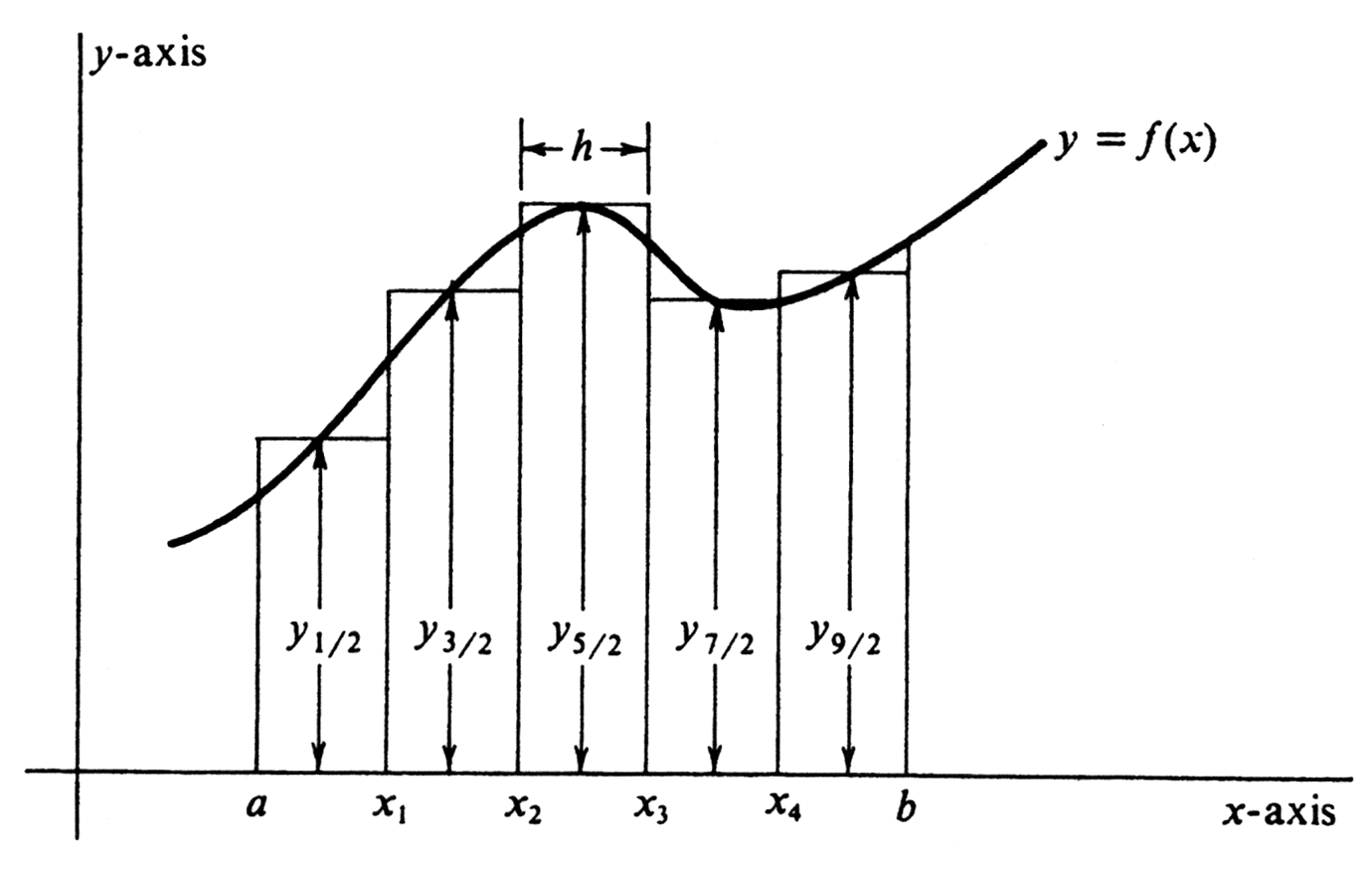
If [math]f(x) \geq 0[/math] for every [math]x[/math] in [math][a, b][/math], the Midpoint Rule approximates the integral [math]\int_a^b f[/math], which is the area under the curve, by a sum of areas of rectangles, as illustrated in Figure 6.

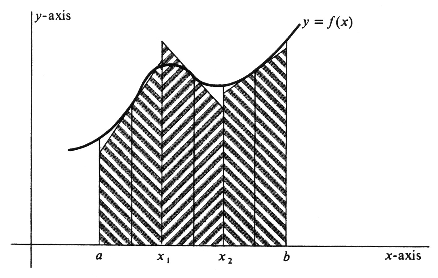
An alternative to approximating the integral by a Riemann sum is to use straight-line segments which are tangent to the curve [math]y = f(x)[/math] at the midpoints of the subintervals. An example is shown in Figure 7, in which

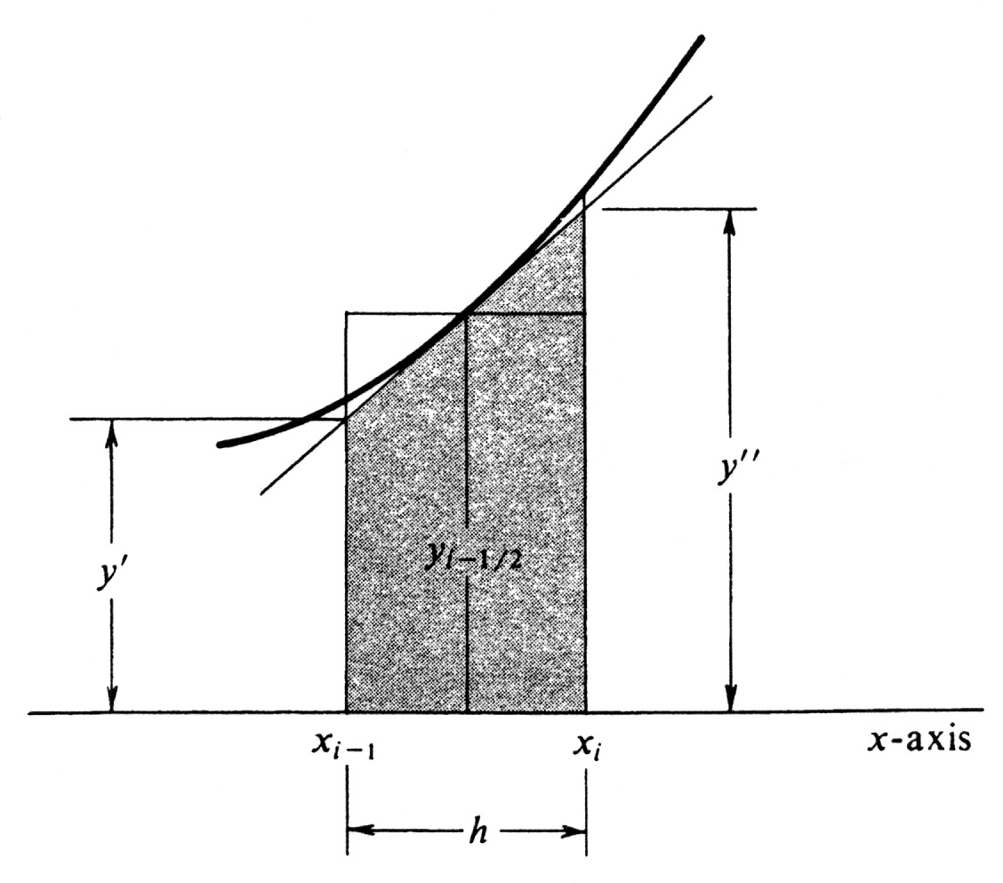
[math]\int_a^b f[/math] is approximated by the sum of the areas of the three shaded trapezoids. This method yields the so-called Tangent Formula. It turns out, however, that the Tangent Formula is the same as the Midpoint Rule. The reason can be seen by looking at Figure 8, in which the area of the shaded trapezoid with one side tangent to the curve is the ith term in the approximating sum used in the Tangent Formula. The area of this trapezoid is equal to [math]\frac{h}{2} (y' + y'')[/math], where [math]y'[/math] and [math]y''[/math] are the lengths of the bases. However, by elementary geometry the trapezoid can be seen to have the same area as the rectangle with base [math][x_{i-1}, x_i][/math] and altitude [math]y_{i-1/2}[/math] The area of the rectangle is [math]h \cdot y_{i-1/2}[/math], and so

[[math]] \frac{h}{2} (y' + y'') = h \cdot y_{i-1/2}. [[/math]]

(Incidentally, note that this equation is true regardless of whether [math]y'[/math], [math]y''[/math], and [math]y_{i-1/2}[/math] are positive, negative, or zero.) Since the product [math]h \cdot y_{i-1/2}[/math] is the ith term in the midpoint approximation [math]M_n[/math], we conclude that the Tangent Formula and the Midpoint Rule, although differently motivated, are in fact the same.

Example

Approximate [math]\int_{-1}^1 (x^2 + x^3) dx[/math] using the Midpoint Rule. This is the same integral which we evaluated in Section 2 by the Trapezoid Rule. To compare the two methods, we shall again take [math]n = 8[/math] and

[[math]] h = \frac{1- (-1)}{8} = \frac{1}{4}. [[/math]]

Since, for an arbitrary interval [math][a, b][/math], we have

[[math]] x_i = a + ih, \;\;\; i = 0, ... ,n, [[/math]]

it follows that

[[math]] \begin{eqnarray*} x_i^{*} &=& \frac{x_{i-1} + x_i}{2} = \frac{[a + (i - 1)h] + (a + ih)}{2}\\ &=& a + (i - \frac{1}{2})h \end{eqnarray*} [[/math]]

In addition, since [math]y_{i-1/2} = f(x_i^{*})[/math], we have a pair of useful formulas:

[[math]] \begin{array}{rl} x_i^{*} &= a + (i - \frac{1}{2})h \\ y_{i-1/2} &= f(a + (i - \frac{1}{2})h) \end{array} \} i = 1, ... , n. [[/math]]

In the present example, [math]a = -1[/math], [math]h = \frac{1}{4}[/math], and [math]f(x) = x^2 + x^3[/math]. Hence

[[math]] \begin{eqnarray*} x_i^{*} &=& -1 + (i - \frac{1}{2})\frac{1}{4} = \frac{2i - 9}{8}, \\ y_{i- 1/2} &=& \Bigl( \frac{2i - 9}{8} \Bigr)^2 + \Bigl( \frac{2i - 9}{8} \Bigr)^3 = \frac{8(2i - 9)^2 + (2i - 9)^3}{8^3} \\ &=& \frac{(2i - 9)^2(2i - 1)}{8^3} . \end{eqnarray*} [[/math]]

Table 2 contains the numbers for the computation of [math]M_8[/math].

[math]i[/math]	[math]y_{i - 1/2} = \frac{(2i - 9)^2(2i - 1)}{8^3}[/math]
1	[math]y_{1/2} = \frac{49}{8^3}[/math]
2	[math]y_{3/2} = \frac{25 \cdot 3}{8^3} = \frac{75}{8^3}[/math]
3	[math]y_{5/2} = \frac{9 \cdot 5}{8^3} = \frac{45}{8^3}[/math]
4	[math]y_{7/2} = \frac{7}{8^3}[/math]
5	[math]y_{9/2} = \frac{9}{8^3}[/math]
6	[math]y_{11/2} = \frac{9 \cdot 11}{8^3} = \frac{99}{8^3}[/math]
7	[math]y_{13/2} = \frac{25 \cdot 13}{8^3} = \frac{325}{8^3}[/math]
8	[math]y_{15/2} = \frac{49 \cdot 15}{8^3} = \frac{735}{8^3}[/math]

Hence we obtain

[[math]] \begin{eqnarray*} M_8 &=& \frac{1}{4}(y_{1/2} + \cdots + y_{15/2})\\ &=& \frac{1}{4 \cdot 8^3} (49 + 75 + 45 + 7 + 9 + 99 + 325 + 735) \\ &=& \frac{1344}{ 4 \cdot 8^3} = \frac{21}{32} \end{eqnarray*} [[/math]]

as an approximation to the integral [math]\int_{-1}^1 (x^2 + x^3) dx[/math]. The value obtained earlier with the Trapezoid Rule was [math]T_8 = \frac{11}{16}[/math]. Since the true value is given by

[[math]] \int_{-1}^1 (x^2 + x^3) dx = \frac{2}{3}, [[/math]]

it follows that the error using the Midpoint Rule is equal to

[[math]] | \frac{2}{3} - \frac{21}{32} | = \frac{1}{96} . [[/math]]

This is one half the error obtained using the Trapezoid Rule with the same value of [math]h[/math].

In any application of the Midpoint Rule, the error [math]| \int_a^b f - M_n |[/math] can be made arbitrarily small by taking [math]n[/math] sufficiently large. That is, we assert that

Theorem

[[math]] \lim_{n \rightarrow \infty} M_n = \int_a^b f . [[/math]]

This theorem is easier to prove than the corresponding one for the Trapezoid Rule because every approximation [math]M_n[/math] is, as it stands, a Riemann sum of [math]f[/math] relative to the partition [math]\sigma_n[/math] of [math][a, b][/math]. Since [math]|| \sigma_n || \rightarrow 0[/math] as [math]n \rightarrow \infty[/math], it is a direct corollary of the fundamental theorem on the limit of Riemann sums [(2.1), page 414] that [math]\lim_{n \rightarrow \infty} M_n = \int_a^b f[/math]. A means of estimating the error [math]| \int_a^b f - M_n |[/math] in a particular application of the Midpoint Rule is provided by the following theorem:

Theorem

If the second derivative [math]f''[/math] is continuous at every point of [math][a, b][/math], then there exists a number [math]c[/math] such that [math]a \lt c \lt b[/math] and

[[math]] \int_a^b f = M_n + \frac{b - a}{24} f''(c) h^2. [[/math]]

As with the analogous theorem for the Trapezoid Rule [(2.4), page 419], this theorem can be proved by first reducing it to the case [math]n = 1[/math]. A discussion of the error term can be found in [math]R[/math]. Courant and F. John, Introduction to Calculus and Analysis, Volume I, Interscience Publishers (Wiley), 1965, pages 486 and 487. Theorem (3.3) can be used to obtain an upper bound on the error [math]|\int_a^b f - M_n|[/math] provided the second derivative [math]f''[/math] is bounded on the interval [math][a, b][/math]. That is, if there exists a real number [math]K[/math] such that

[[math]] | f''(x) | \leq K, \;\;\; \mbox{for every $x$ in $[a, b]$,} [[/math]]

then, in particular [math]|f''(c)| \leq K[/math], and so

[[math]] \begin{eqnarray*} \Big| \int_a^b f - M_n \Big| &=& \frac{(b - a)h^2}{24} | f''(c) | \\ &\leq& \frac{(b - a)K}{24} h^2 . \end{eqnarray*} [[/math]]

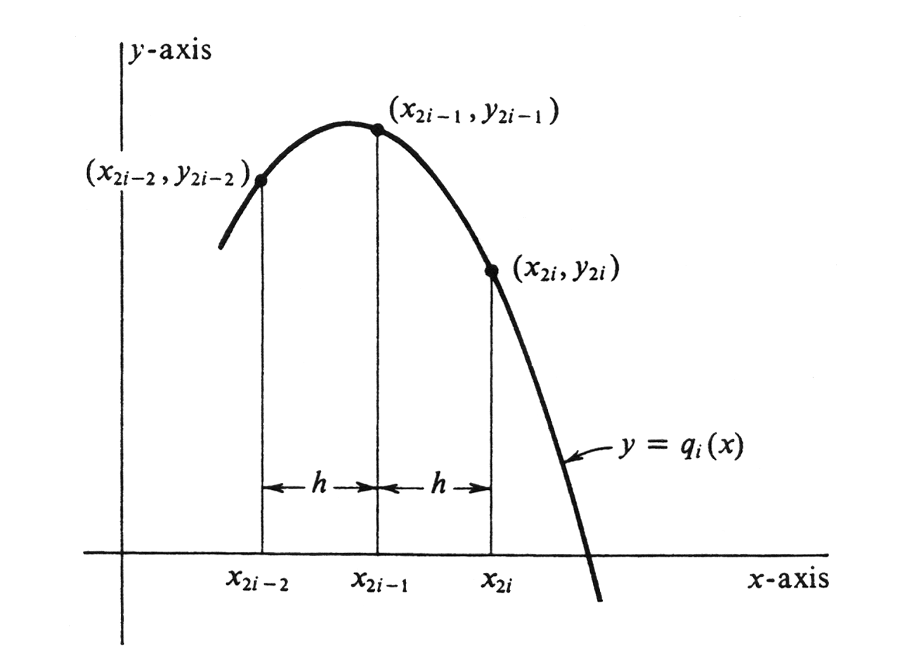
For the one integral we computed by both methods, the Midpoint Rule gave a better approximation than the Trapezoid Rule by a factor of 2. Comparison of Theorem (3.3) with (2.4) shows that in general this ratio can be expected. Geometrically, the different methods of numerical integration described thus far in this and the preceding section are all based on approximating the area under a curve by a sum of areas of rectangles or trapezoids. Analytically, in each method the approximation to [math]\int_a^b f[/math] has been obtained by replacing [math]f[/math] over every subinterval by a linear function. In Simpson's Rule, however, we shall replace [math]f[/math] over each subinterval by a quadratic polynomial [math]Ax^2 + Bx + C[/math]. The corresponding area problem is the simple one of finding the area under a parabola (or a straight line, if [math]A = 0[/math]). For most integrals, Simpson's Rule gives much greater accuracy for the same value of [math]h[/math]. Let [math]f[/math] be a function which is integrable over the interval [math][a, b][/math]. The procedure differs from the others in that we consider only partitions of [math][a, b][/math] into an even number of subintervals. Thus for an arbitrary even integer [math]n \gt 0[/math], we set [math]h = \frac{b - a}{n}[/math], and let

[[math]] \begin{eqnarray*} x_i &=& a + ih,\\ y_i &=& f (x_i), \;\;\; \mbox{for}\; i = 0, . . ., n. \end{eqnarray*} [[/math]]

Since [math]n[/math] is even, there is an integral number of “double” intervals [math][x_{2i-2}, x_{2i}], i = 1, ... , \frac{n}{2}[/math] as illustrated in Figure 9, and

[[math]] \int_a^b f(x) dx= \sum_{i=1}^{n/2} \int_{x_{2i-2}}^{x_{2i}} f(x) dx. [[/math]]

There exists one and only one polynomial [math]q_i(x) = A_i x^2 + B_i x + C_i[/math] of degree less than three whose graph passes through the three points [math](x_{2i-2}, y_{2i-2}), (x_{2i-1}, y_{2i-1})[/math], and [math](x_{2i}, y_{2i})[/math] (see Figure 10). Over each double interval [math][x_{2i-2}, x_{2i}][/math] we shall approximate the integral of [math]f[/math] by the integral of [math]q_i[/math]. Let us assume for the moment, and later prove, the fact that

[[math]] \begin{equation} \int_{x_{2i-2}}^{x_{2i}} q_i(x) dx = \frac{h}{3} (y_{2i-2} + 4y_{2i-1} + y_{2i}). \label{eq8.3.1} \end{equation} [[/math]]

The sum of these integrals, which we shall denote [math]S_n[/math], is the approximation to [math]\int_a^b f[/math] prescribed by Simpson's Rule. Hence

[[math]] S_n = \frac{h}{3} \sum_{i=1}^{n/2} (y_{2i-2} + 4y_{2i-1} + y_{2i}) . [[/math]]

If this sum is expanded, note the pattern of the coefficient of the [math]y_i[/math]'s: If [math]i[/math] is odd, the coefficient of [math]y_i[/math] is 4. If [math]i[/math] is even, the coefficient is 2, with the exception of [math]y_0[/math] and [math]y_n[/math], each of which has coefficient 1. Thus Simpson's Rule is expressed in the formula

Theorem

[[math]] \begin{eqnarray*} \int_a^b f \approx S_n &=& \frac{h}{3} (y_0 + 4y_1 + 2y_2 + 4y_3 + 2y_4\\ && + \cdots + 2y_{n-2} + 4y_{n-1} + y_n) . \end{eqnarray*} [[/math]]

We now prove equation (1). The algebra is significantly simpler if we write [math]q_{i}(x)[/math] in terms of [math]x - x_{2i-1}[/math] instead of [math]x[/math] (see Figure 10). Hence we let

[[math]] \begin{equation} q_i(x) = \alpha_i(x - x_{2i-1})^2 + \beta_i(x- x_{2i-1}) + \gamma_i. \label{eq8.3.2} \end{equation} [[/math]]

The integral [math]\int_{x_{2i-2}}^{x_{2i}} q_i (x) dx[/math] may be computed by substituting [math]u = x - x_{2i-1}[/math] and using the Change of Variable Theorem for Definite Integrals (see page 215). Since [math]x_{2i-2} - x_{2i-1} = - h[/math] and [math]x_{2i} - x_{2i-1} = h[/math], the result is

[[math]] \begin{equation} \begin{array}{ll} \int_{x_{2i-2}}^{x_{2i}} q_i (x) dx &= \int_{-h}^h (\alpha_i u^2 + \beta_i u + \gamma_i) du \\ &= \Bigl( \frac{\alpha_i u^3}{3} + \frac{\beta_i u^2}{2} + \gamma_i u \Bigr) \big|_{-h}^h \\ &= \frac{h}{3} (2\alpha_i h^2 + 6\gamma_i). \end{array} \label{eq8.3.3} \end{equation} [[/math]]

Setting first [math]x = x_{2i-1}[/math] in equation (2), we obtain

[[math]] y_{2i-1} = q_i(x_{2i-1}) = \alpha_i \cdot 0^2 + \beta_i \cdot 0 + \gamma_i = \gamma_i. [[/math]]

Next we let [math]x = x_{2i-2}[/math] and [math]x = x_{2i}[/math] to get

[[math]] y_{2i-2} = q_i(x_{2i-2}) = \alpha_i h^2 - \beta_{i}h + \gamma_i, [[/math]]

and

[[math]] y_{2i} = q_i(x_{2i}) = \alpha_i h^2 + \beta_i h + \gamma_i. [[/math]]

Adding, we obtain

[[math]] y_{2i-2} + y_{2i} = 2\alpha_i h^2 + 2\gamma_i. [[/math]]

Since [math]\gamma_i = y_{2i-1}[/math], it follows that

[[math]] 2\alpha_i h^2 + 6\gamma_i = y_{2i-2} + 4y_{2i-1} + y_{2i}. [[/math]]

Substituting this result in (3) yields the desired result (1), and the derivation of Simpson's Rule is complete.

Example

Using [math]n = 4[/math], find an approximate value of [math]\int_0^1 \frac{1}{1+ x^2} dx[/math] by Simpson's Rule. We have [math]h = \frac{1 - 0}{4} = \frac{1}{4}[/math],

[[math]] \begin{eqnarray*} x_i &=& \frac{i}{4}, \;\;\; i = 0,1,..., 4,\\ y_i &=& \frac{1}{1 + x_i^2} = \frac{1}{1 + \frac{i^2}{16}} = \frac{16}{16 + i^2}, \;\;\; i = 0, 1,..., 4. \end{eqnarray*} [[/math]]

Table 3 contains the numbers necessary for the computation.

[math]i[/math]	0	1	2	3	4\vspace {1ex}
[math]y_i = \frac{16}{16 + i^2}[/math]	1	[math]\frac{16}{17}[/math]	[math]\frac{16}{20}[/math]	[math]\frac{16}{25}[/math]	[math]\frac{16}{32}[/math] \vspace {1ex}

Hence

[[math]] \begin{eqnarray*} S_4 &=& \frac{h}{3} - (y_0 + 4y_1 + 2y_2 + 4y_3 + y_4)\\ &=& \frac{1}{12} (1 + \frac{64}{17} + \frac{32}{20} + \frac{64}{25} + \frac{16}{32}) \\ &=& 0.785392.... \end{eqnarray*} [[/math]]

We know that

[[math]] \int_0^1\frac{1}{1 + x^2} dx = \arctan x \big|_0^1 = \frac{\pi}{4} = 0.785398.... [[/math]]

Hence the error [math]|\int_a^b f - S_4|[/math] is approximately 0.000006.

Just as with the other two methods of integration by numerical approximation, the error [math]| \int_a^b f - S_n |[/math] can be made arbitrarily small by taking [math]n[/math] aufficiently large. That is, we have the following theorem, which we state without proof.

Theorem

[[math]] \lim_{n \rightarrow \infty} S_n = \int_a^b f . [[/math]]

In addition, the next theorem can be used to estimate the error in a particular application of Simpson's Rule.

Theorem

If the fourth derivative [math]f^{(4)}[/math] is continuous at every point of [math][a, b][/math], then there exists a number [math]c[/math] such that [math]a \lt c \lt b[/math] and

[[math]] \int_a^b f = S_n - \frac{b - a}{180} f^{(4)} (c)h^4. [[/math]]

For an outline of a proof, see J. M. H. Olmsted, Advanced Calculus, Appleton-Century-Crofts, 1961, page 119. The fourth derivative of every cubic polynomial is identically zero, for if

[[math]] f(x) = a_{3}x^3 + a_{2}x^2 + a_{1}x + a_0, [[/math]]

then [math]f^{(4)} (x) = 0[/math]. It is therefore a rather surprising corollary of Theorem(3.6) that Simpson's Rule will always give the exact value of the integral when applied to any polynomial of degree less than 4.

General references

Doyle, Peter G. (2008). "Crowell and Slesnick's Calculus with Analytic Geometry" (PDF). Retrieved Oct 29, 2024.