The Central limit theorem (real case)
Let [math] (\Omega,\A,\p) [/math] be a probability space. Let [math] (X_n)_{n\geq 1} [/math] be a sequence of iid r.v.'s with values in [math] \R [/math] . We assume that [math] \E[X_k^2] \lt \infty [/math] (i.e. [math] X_k\in L^2(\Omega,\A,\p) [/math] ) and let [math] \sigma^2=Var(X_k) [/math] for all [math] k\in\{1,...,n\} [/math] . Then for all [math] k\in\{1,...,n\} [/math] we get
Without loss of generality we can assume that [math] \E[X_k]=0 [/math] , for all [math] k\in\{1,...,n\} [/math] . Define now a sequence [math] Z_n=\frac{\sum_{i=1}^nX_i}{\sqrt{n}} [/math] . Then we can obtain
Example
If [math]\E[X_k]=0[/math] for all [math]k\in\{1,...,n\}[/math], then


Let [math](X_n)_{n\geq 1}[/math] be independent r.v.'s but not necessarily i.i.d. We assume that [math]\E[X_j]=0[/math] and that [math]\E[X_j^2]=\sigma_j^2 \lt \infty[/math], for all [math]j\in\{1,...,n\}[/math]. Assume further that [math]\sup_n\E[\vert X_n\vert^{2+\delta}] \lt \infty[/math] for some [math]\delta \gt 0[/math], and that [math]\sum_{j=1}^\infty \sigma_j^2 \lt \infty.[/math] Then
Example
We got the following examples:
- Let [math](X_n)_{n\geq 1}[/math] be i.i.d. r.v.'s with [math]\p[X_n=1]=p[/math] and [math]\p[X_n=0]=1-p[/math]. Then [math]S_n=\sum_{i=1}^nX_i[/math] is a binomial r.v. [math]\B(p,n)[/math]. We have [math]\E[S_n]=np[/math] and [math]Var(S_n)=np(1-p)[/math]. Now with the strong law of large numbers we get [math]\frac{S_n}{n}\xrightarrow{n\to\infty\atop a.s.}p[/math] and with the central limit theorem we get
[[math]] \frac{S_n-np}{\sqrt{np(1-p)}}\xrightarrow{n\to\infty\atop law}\mathcal{N}(0,1). [[/math]]
- Let [math]\mathcal{P}[/math] be the set of prime numbers. For [math]p\in\mathcal{P}[/math], define [math]\B_p[/math] as [math]\p[\B_p=1]=\frac{1}{p}[/math] and [math]\p[\B_p=0]=1-\frac{1}{p}[/math]. We take the [math](\B_p)_{p\in\mathcal{P}}[/math] to be independent and
[[math]] W_n=\sum_{\mathcal{P}\subset\N\atop p\in\mathcal{P}}\B_p, [[/math]]the probabilistic model for the total numbers of distinct prime divisors of [math]n:=W(0)[/math]. It's a simple exercise to check that [math](W_n)_{n\geq 1}[/math] satisfies the assumption of theorem 13.2 and using the fact that [math]\sum_{p\leq n\atop p\in\mathcal{P}}\frac{1}{p}\sim \log\log n[/math] and we obtain[[math]] \frac{W_n-\log\log n}{\sqrt{\log\log n}}\xrightarrow{n\to\infty\atop law}\mathcal{N}(0,1). [[/math]]
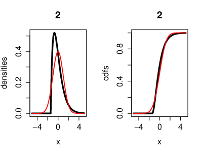
An illustration of the CLT, where the r.v.'s [math](X_n)[/math] are i.i.d. exponentially distributed. Also with the cumulative distribution functions. Here we have [math]n=2[/math] exponentially distributed r.v's [math]\left(X_k\sim \lambda e^{-\lambda}\right)[/math]. On the left side, the black curve represents the density function of the r.v.'s and the red curve represents the density of a Gaussian r.v. [math]Y[/math] with [math]\mu=0[/math] ([math]Y\sim\mathcal{N}(0,\sigma^2)[/math]). On the right side, the black curve represents the cumulative distribution function of the r.v.'s [math]X_k[/math] and the red curve represents the cumulative distribution function of a Gaussian r.v. [math]Y[/math]. 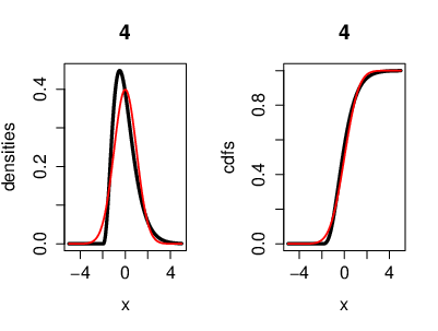
An illustration of the CLT, where the r.v.'s [math](X_n)[/math] are i.i.d. exponentially distributed. Also with the cumulative distribution functions. Here we have [math]n=4[/math] exponentially distributed r.v's [math]\left(X_k\sim \lambda e^{-\lambda}\right)[/math]. On the left side, the black curve represents the density function of the r.v.'s and the red curve represents the density of a Gaussian r.v. [math]Y[/math] with [math]\mu=0[/math] ([math]Y\sim\mathcal{N}(0,\sigma^2)[/math]). On the right side, the black curve represents the cumulative distribution function of the r.v.'s [math]X_k[/math] and the red curve represents the cumulative distribution function of a Gaussian r.v. [math]Y[/math]. 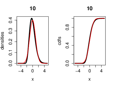
An illustration of the CLT, where the r.v.'s [math](X_n)[/math] are i.i.d. exponentially distributed. Also with the cumulative distribution functions. Here we have [math]n=10[/math] exponentially distributed r.v's [math]\left(X_k\sim \lambda e^{-\lambda}\right)[/math]. On the left side, the black curve represents the density function of the r.v.'s and the red curve represents the density of a Gaussian r.v. [math]Y[/math] with [math]\mu=0[/math] ([math]Y\sim\mathcal{N}(0,\sigma^2)[/math]). On the right side, the black curve represents the cumulative distribution function of the r.v.'s [math]X_k[/math] and the red curve represents the cumulative distribution function of a Gaussian r.v. [math]Y[/math]. 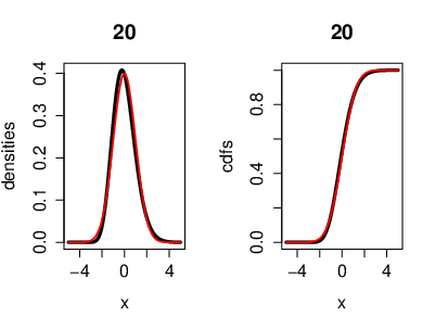
An illustration of the CLT, where the r.v.'s [math](X_n)[/math] are i.i.d. exponentially distributed. Also with the cumulative distribution functions. Here we have [math]n=20[/math] exponentially distributed r.v's [math]\left(X_k\sim \lambda e^{-\lambda}\right)[/math]. On the left side, the black curve represents the density function of the r.v.'s and the red curve represents the density of a Gaussian r.v. [math]Y[/math] with [math]\mu=0[/math] ([math]Y\sim\mathcal{N}(0,\sigma^2)[/math]). On the right side, the black curve represents the cumulative distribution function of the r.v.'s [math]X_k[/math] and the red curve represents the cumulative distribution function of a Gaussian r.v. [math]Y[/math]. Now we can see that both, the density and the cumulative distribution function, are converging to a Gaussian density and a Gaussian cumulative distribution function for [math]n\to\infty[/math]. Theorem (Erdös-Kac)Let [math]N_n[/math] be a r.v. with uniformly distribution in [math]\{1,...,n\}[/math], then
[[math]] \frac{W(N_n)-\log\log n}{\sqrt{\log\log n}}\xrightarrow{n\to\infty\atop law}\mathcal{N}(0,1), [[/math]]where [math]W(n)=\sum_{p\leq n\atop p\in\mathcal{P}}\one_{p|n}[/math]. - Suppose that [math](X_n)_{n\geq 1}[/math] are i.i.d. r.v.'s with distribution function [math]F(x)=\p[X_1\leq x][/math]. Let [math]Y_n(x)=\one_{X_n\leq x}[/math], where [math](Y_n)_{n\geq 1}[/math] are i.i.d. Define [math]F_n(x)=\frac{1}{n}\sum_{k=1}^nY_k(x)=\frac{1}{n}\sum_{k=1}^n\one_{X_k\leq x}[/math]. [math]F_n[/math] is called the empirical distribution function. With the strong law of large numbers we get [math]\lim_{n\to\infty\atop a.s.}F_n(x)=\E[Y_1(x)][/math] and
[[math]] \E[Y_1(x)]=\E[\one_{X_1\leq x}]=\p[X_1\leq x]=F(x). [[/math]]In fact, it is a theorem (Gliwenko-Cantelli) which says that[[math]] \sup_{x\in\R}\vert F_n(x)-F(x)\vert\xrightarrow{n\to\infty\atop a.s.}0. [[/math]]Next we note that[[math]] \sqrt{n}(F_n(x)-F(x))=\sqrt{n}\left(\frac{1}{n}\sum_{k=1}^nY_k(x)-\E[Y_1(x)]\right)=\frac{1}{\sqrt{n}}\left(\sum_{k=1}^nY_k(x)-n\E[Y_1(x)]\right) [[/math]]Now with the central limit theorem we get[[math]] \sqrt{n}(F_n(x)-F(x))\xrightarrow{n\to\infty\atop law}\mathcal{N}(0,\sigma^2(x)), [[/math]]where [math]\sigma^2(x)=Var(Y_1)=\E[Y_1^2(x)]=\E[Y_1(x)]=F(x)-F^2(x)=F(x)(1-F(x))[/math]. Hence[[math]] \sqrt{n}(F_n(x)-F(x))\xrightarrow{n\to\infty\atop law}\mathcal{N}(0,F(x)(1-F(x))). [[/math]]


Let [math](X_n)_{n\geq 1}[/math] be i.i.d. r.v's and suppose that [math]\E[\vert X_k\vert^3] \lt \infty[/math], [math]\forall k\in\{1,...,n\}[/math]. Let
where [math]\sigma^2=\E[X_k^2][/math] [math]\forall k\in\{1,...,n\}[/math] and [math]\Phi(x)=\p\left[\mathcal{N}(0,1)\leq x\right]=\int_{-\infty}^xe^{-\frac{u^2}{2}}\frac{1}{\sqrt{2\pi}}du[/math]. Then
General references
Moshayedi, Nima (2020). "Lectures on Probability Theory". arXiv:2010.16280 [math.PR].