Separating Gaussian data
After having studied in previous chapters the properties of high-dimensional data that comes from a Gaussian distribution, we now want use this knowledge to understand under which conditions it is possible to separate (or ‘disentangle’) the data that stems from two ‘Gaussians’ with variance one and different means. Let us first look at low dimensions, for example at the 2-dimensional data set in Figure, which we generated by drawing samples of equal size from two Gaussians with different centers.
Separation (or disentanglement) in Figure would mean to determine for each point if it came from the lower left Gaussian or from the upper right Gaussian. Firstly, we observe that this cannot be done in a deterministic way but only ‘with high probability for almost all points’. Secondly we see, that for this to be possible it is necessary that the distance between the two means is sufficiently large. If this is the case, we might have a good chance that pairs of data points with small distances belong to the same Gaussian whereas pairs with large distances belong to different Gaussians. Moreover, there will be only a few points located half way between the centers which means that if we start by picking an arbitrary data point and then compute the other points' distances from the fixed one, we may expect that two clusters, corresponding to the two Gaussians, appear.
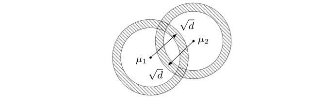
In high dimensions the picture looks different. We know that here most data points of a Gaussian are located in an annulus with radius [math]\sqrt{d}[/math] around the mean of the Gaussian. An analogue of the assumption in the 2-dimensional case would thus require that the distance [math]\Delta:=\|\mu_1-\mu_2\|[/math] between the means is larger than [math]2\sqrt{d}[/math], see Figure, implying that the data sets will be almost disjoint. \begin{center}
If this is the case, then we may expect that separation can be done analogously to the low-dimensional situation. There are however two principal differences: Firstly, our asymptotic approach to high dimensions means that we do not consider [math]d[/math] as a constant but always ask what happens for [math]d\rightarrow\infty[/math]. Therefore, we need to understand the distance of the means [math]\Delta=\Delta(d)[/math] as a function of the dimension as well. Otherwise, i.e., for constant [math]\Delta[/math] and dimension tending to infinity, the two annuli would eventually overlap more and more and become almost coincident. From this we see that we have to require that [math]\Delta\rightarrow\infty[/math]. Our low-dimensional arguments suggest that [math]\Delta \gt 2\sqrt{d}[/math] yields one scenario in which disentanglement can be achieved. On the other hand, the picture in Figure suggests that the overlap might also be small, even if [math]\Delta\leqslant2\sqrt{d}[/math].
We emphasize that Figure and in particular Figure constitute rather imperfect 2-dimensional abstract illustrations of high dimensional facts. Notice, e.g., that any two points in one of the annuli have, with high probability, distance [math]\sqrt{2d}[/math]. The picture does however not represent this at all!
Notice that also in this second scenario [math]\Delta\rightarrow\infty[/math] must hold in order to avoid that for large [math]d[/math] the the two annuli become almost coincident. The picture suggests nevertheless that this can be achieved also for [math]\Delta[/math]'s that grow slower than [math]2\sqrt{d}[/math] and experiments corroborate this idea. For Figure below we considered two Gaussians in dimension [math]d=1000[/math], sampled 100 points from each of them, and plotted the distribution of the sample's mutual distances.

Indeed, the distances of points that belong to the same Gaussian accumulate around [math]\sqrt{2d}\approx44.72[/math]. This suggests that the other ‘bump’ in the picture belongs to those pairs of points which come from different Gaussians. In our example we have a distance of [math]\Delta\approx31.62[/math] between the Gaussians' centers and [math]2\sqrt{d}\approx63.25[/math]. This shows that we are in the situation of Figure, i.e., the Gaussians overlap. The distribution of mutual distances suggest that it nevertheless should be possible to disentangle them with high accuracy. Indeed, if we pick for a start one point at random and then take its 100 nearest neighbors, Figure suggests that our odds are good that these 100 points will belong to one of the Gaussians and the rest of the points to the other.
Our aim now is to make the above formal. We start by computing the expected values for the distance between points that belong to different Gaussians.
Let [math]\mu_1[/math], [math]\mu_2\in\mathbb{R}^d[/math] and [math]\Delta:=\|\mu_1-\mu_2\|[/math]. Let [math]X_1\sim\mathcal{N}(\mu_1,1,\mathbb{R}^d)[/math] and [math]X_2\sim\mathcal{N}(\mu_2,1,\mathbb{R}^d)[/math] be random vectors.
- [math]\forall\:d\geqslant1\colon\bigl|\E\bigl(\|X_1-X_2\|-\sqrt{\Delta^2+2d}\bigr)\bigr|\leqslant \medfrac{3d+8\Delta^2+\sqrt{24}\Delta d^{1/2}}{2(\Delta^2+2d)^{3/2}}[/math].
- [math]\forall\:d\geqslant1\colon\V(\|X_1-X_2\|)\leqslant \Bigl(\medfrac{3d+8\Delta^2+\sqrt{24}\Delta d^{1/2}}{2(\Delta^2+2d)^{3/2}}\Bigr)^2 + \medfrac{3d+8\Delta^2+\sqrt{24}\Delta d^{1/2}}{\Delta^2+2d}[/math].
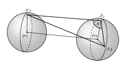
(i) Let [math]X_1[/math], [math]X_2\colon\Omega\rightarrow\mathbb{R}^d[/math] be as above. We define the auxiliary random vector [math]\tilde{X}_1:=\mu_2+X_1-\mu_1[/math]. Then [math]\tilde{X}_1\sim\mathcal{N}(\mu_2,1,\mathbb{R}^d)[/math] holds. Moreover, [math]\tilde{X}_1[/math] and [math]X_2[/math] are independent. For a fixed [math]\omega\in\Omega[/math] we get the following picture for the values [math]x_1:=X_1(\omega)[/math], [math]x_2:=X_2(\omega)[/math] and [math]\tilde{x}_1:=\tilde{X}_1(\omega)\in\mathbb{R}^d[/math]. Firstly, in view of Theorem we may assume that [math]x_1[/math] will be located near the surface of a ball with radius [math]\sqrt{d}[/math] centered at [math]\mu_1[/math] and that [math]x_2[/math] and [math]\tilde{x}_1[/math] will both be located near the surface of a ball with radius [math]\sqrt{d}[/math] centered at [math]\mu_2[/math]. By definition of [math]\tilde{x}_1[/math] the lines connecting [math]\mu_1[/math] with [math]x_1[/math] and [math]\mu_2[/math] with [math]\tilde{x}_1[/math], respectively, will be parallel. Moreover, if we think of a coordinate system in which [math]\mu_2[/math] is the origin, then we may expect that [math]\tilde{x}_1[/math] and [math]x_2[/math] have a distance of approximately [math]\sqrt{2d}[/math], compare Theorem. Finally, we think of the line going from [math]\mu_2[/math] to [math]\mu_1[/math] marking the north pole of [math]\B(\mu_2,\sqrt{d})[/math]. Then Theorem suggests that [math]\tilde{x}_1[/math] and [math]x_2[/math] will be located close to the equator of [math]\B(\mu_2,\sqrt{d})[/math], since the scalar products [math]\langle{}\tilde{x}_1-\mu_2,\mu_1-\mu_2\rangle{}[/math] and [math]\langle{}x_2-\mu_2,\mu_1-\mu_2\rangle{}[/math] both will be close to zero. In the triangle given by all three points we thus may expect that the angle [math]\theta[/math] will be close to [math]90^{\circ}[/math] which implies that [math]\|x_1-x_2\|^2\approx\Delta^2+2d[/math] should hold.

Following the above intuition, we will now formally use the cosine law and our results from Chapter The curse of high dimensions to compute the expectation. We put [math]\xi:=\mu_1-\mu_2[/math] and start with
(ii) Finally we get
In the following results we understand [math]\Delta=\Delta(d)[/math] as a function of the dimension. To keep the notation short we will however drop the ‘of [math]d[/math]’ most of the time.
Let [math]\mu_1[/math], [math]\mu_2\in\mathbb{R}^d[/math] and [math]\Delta:=\|\mu_1-\mu_2\|[/math]. Let [math]X_1\sim\mathcal{N}(\mu_1,1,\mathbb{R}^d)[/math] and [math]X_2\sim\mathcal{N}(\mu_2,1,\mathbb{R}^d)[/math] be random variables. Assume either that there exists [math]d_0\geqslant1[/math] such that [math]\Delta\geqslant2\sqrt{d}[/math] holds for all [math]d\geqslant d_0[/math] or that there exists [math]d_0\geqslant1[/math] such that [math]\Delta \lt 2\sqrt{d}[/math] holds for all [math]d\geqslant d_0[/math]. Then
We start with the first scenario, assume [math]\Delta\geqslant2\sqrt{d}[/math], i.e., [math]d\leqslant\Delta^2/4[/math], and estimate
The above suggests that if we pick two points [math]x[/math] and [math]y[/math] from Gaussians with different centers at random, then we have to expect that [math]\|x-y\|\approx\sqrt{\Delta^2+2d}[/math] holds for large [math]d[/math] and that the distribution does not spread out when [math]d[/math] increases. On the other hand we know already from Chapter The curse of high dimensions that [math]\|x-y\|\approx\sqrt{2d}[/math] for large [math]d[/math] provided that [math]x[/math] and [math]y[/math] are sampled from the same Gaussian. This implies that the question if the two Gaussians can be separated, requires that the distance [math]\sqrt{\Delta^2+2d}-\sqrt{2d}[/math] between the two expectational values is large enough. For the two scenarios covered by Corollary we get the following.
Let [math]\Delta\colon\mathbb{N}\rightarrow(0,\infty)[/math] and [math]\delta\colon\mathbb{N}\rightarrow(0,\infty)[/math], [math]\delta(d):=\sqrt{\Delta^2+2d}-\sqrt{2d}[/math].
- If there exists [math]d_0\geqslant1[/math] such that [math]\Delta\geqslant2\sqrt{d}[/math] holds for all [math]d\geqslant d_0[/math], then [math]\delta(d)\geqslant\sqrt{d}[/math] holds for [math]d\geqslant d_0[/math].
- If there exists [math]d_0\geqslant1[/math], [math]c \gt 0[/math] and [math]\alpha\geqslant0[/math] such that [math]cd^{1/4+\alpha}\leqslant\Delta \lt 2\sqrt{d}[/math] holds for all [math]d\geqslant d_0[/math], then [math]\delta(d)\geqslant (c^2/4)d^{2\alpha}[/math] holds for [math]d\geqslant d_0[/math].
(i) In this case we compute
We will see later how Lemma outlines for the situation sketched in Figure, how fast [math]\Delta[/math] needs to grow in order to separate two Gaussians. Before we discuss this, we need however the following explicit probability estimate complementing our results in Theorem and Corollary on expectation and variance.
Let [math]\mu_1[/math], [math]\mu_2\in\mathbb{R}^d[/math] and let [math]\Delta:=\|\mu_1-\mu_2\| \gt 0[/math]. Let [math]x_1[/math] and [math]x_2[/math] be drawn at random with respect to Gaussian distribution with unit variance and means [math]\mu_1[/math] and [math]\mu_2[/math], respectively. Then
Formally, we consider random variables [math]X_i\sim\mathcal{N}(\mu_i,1,\mathbb{R}^d)[/math] for [math]i=1,2[/math] and we estimate
The following is the core result on separability as we can use it to see that points which have ‘small’ mutual distance belong to the same Gaussian with high probability.
(Separation Theorem) Let [math]\mu_1[/math], [math]\mu_2\in\mathbb{R}^d[/math] and put [math]\Delta:=\|\mu_1-\mu_2\|[/math]. Let [math]\epsilon_1 \gt 18[/math] and [math]\epsilon_2 \gt 54[/math] be constant and assume that there is [math]d_0\geqslant1[/math] such that [math]\sqrt{\Delta^2+2d}-\sqrt{2d} \gt \epsilon_1+\epsilon_2[/math] holds for [math]d\geqslant d_0[/math]. Let [math]X_i\sim\mathcal{N}(\mu_i,1,\mathbb{R}^d)[/math] and [math]S_i:=\{x_i^{\scriptscriptstyle(1)},\dots,x_i^{\scriptscriptstyle(n)}\}[/math] be samples of [math]X_i[/math] for [math]i=1,2[/math] such that [math]S_1\cap S_2=\emptyset[/math]. Let [math]x,y\in S_1\cup S_2[/math]. Then
On the basis of our prior experiments, see Figure, and in view of Theorem and Corollary we expect that the mutual distances will accumulate around the values [math]\sqrt{2d}[/math] and [math]\sqrt{\Delta^2+2d}[/math]. Our assumptions imply [math]\sqrt{2d}+\epsilon_1 \lt \sqrt{\Delta^2+2d}-\epsilon_2[/math] which guarantees that [math]\Bbar(\sqrt{2d},\epsilon_1)[/math] and [math]\Bbar(\sqrt{\Delta^2+2d},\epsilon_2)[/math] have empty intersection, i.e., there is some space between the two ‘bumps’ sketched in Figure below.

To keep notation short let us abbreviate [math]x\sim y[/math] for the case that [math]x[/math] and [math]y[/math] come from the same Gaussian, i.e., if [math]x,\,y\in S_1[/math] or [math]x,\,y\in S_2[/math]. Consequently, [math]x\not\sim y[/math] means [math]x\in S_1, y\in S_2[/math] or [math]x\in S_2,\,y\in S_1[/math]. We use Bayes Theorem to compute the conditional probability
Notice that in order to apply Theorem we need that [math]\delta=\sqrt{\Delta^2+2d}-\sqrt{2d}\geqslant\epsilon_1+\epsilon_2 \gt 72[/math] holds. Here, [math]\delta=\delta(d)[/math] can for example be large and bounded or even tend to infinity. If the latter is the case, we may in \eqref{SEP-EQ-1} consider [math]\epsilon_2\rightarrow\infty[/math] as well. We state concrete examples for this below.
Let [math]\epsilon_1 \gt 18[/math] be constant, [math]\epsilon_2=d^{\alpha}[/math] and [math]\Delta=2d^{1/4+\alpha}[/math] with [math]\alpha \gt 0[/math]. Then the assumptions of Theorem are met and we have
We first consider the case [math]\alpha\geqslant1/4[/math]. Then by Lemma(i) we get that [math]\delta\geqslant d^{1/2} \gt \epsilon_1+d^{1/4}[/math] holds for large [math]d[/math]. We may thus proceed as in the proof of the previous theorem and at its end we see, since [math]\epsilon_2\rightarrow\infty[/math] for [math]d\rightarrow\infty[/math], that the limit inferior is bounded from below by [math]1-18/\epsilon_1[/math].
Let now [math]\alpha \lt 1/4[/math]. Then we apply Lemma(ii) and get that [math]\delta\geqslant (2^2/4)d^{2\alpha} \gt \epsilon_1+d^{\alpha}[/math] for large [math]d[/math]. From this point on we can proceed as in the first part.
We conclude this chapter by running the separation algorithm suggested by our previous results with the parameters outlined in Corollary. That is, we consider two [math]d[/math]-dimensional Gaussians whose centers have distance [math]\Delta=\Delta(d)[/math] and sample from each of them 100 points. Then we pick one data point at random and label its 100 nearest neighbors with [math]0[/math], the rest with [math]1[/math]. Finally we check how many of the points with the same label came from the same Gaussian. The charts below show the rate of correctly classified points for different choices of [math]\Delta[/math].

We leave it as Problem to verify the above and we mention that for [math]\Delta=2\sqrt{d}[/math] in experiments the rate of correctly classified points turned out to be one for all dimensions. Finally let us look at the the distribution of mutual distances in a case where [math]\Delta[/math] is (too) small.

The pictures in Figure show the distribution of mutual distances between 200 points sampled from two different Gaussians in [math]\mathbb{R}^{1000}[/math]. In the left picture the distance between their means is 25 and in the right picture it is 30. In the experiment that lead to the right picture our algorithm still correctly classified 98% of the points, whereas in the experiment underlying the left picture we only got 85% right. Notice that the threshold identified in Corollary is [math]2d^{1/4}=20[/math].
General references
Wegner, Sven-Ake (2024). "Lecture Notes on High-Dimensional Data". arXiv:2101.05841 [math.FA].


