Financial Introduction

[math] \newcommand{\indicator}[1]{\mathbbm{1}_{\left[ {#1} \right] }} \newcommand{\Real}{\hbox{Re}} \newcommand{\HRule}{\rule{\linewidth}{0.5mm}} \newcommand{\mathds}{\mathbb}[/math]

\label{sec:intro} In this section we'll discuss some of the basic ideas of option pricing. The main idea is replication, whereby a derivative security can be priced because it is shown to have the same cash flows as a portfolio of assets that already have a price-tag. Another word to describe such a notion of pricing is benchmarking, where to say that you've ‘benchmarked the security’ might mean that you've found a portfolio of other assets that do not replicate but have have some similarities to the derivative's cash flows. The idea of finding a portfolio that is close in value to the derivative security is essentially the law of one price, which states that ‘`In an efficient market, all identical goods must have only one price." Indeed, we will assume that our markets are efficient, and in some cases we will assume that arbitrage has zero probability of occurring; these assumptions are routine and are generally not considered to be restrictive. The manner in which these notes can be considered `oversimplified’ is in the completeness of the resulting markets. In practice there are derivatives (e.g. insurance products) which cannot be hedged, and hence the market is incomplete. Both the discrete time-space market and the Black-Scholes market are simple enough for completeness to hold. In practice, reverse-engineering these models from real-life market data will require interpretation.

A Market in Discrete Time and Space

Consider a very simple market where at time [math]t=0[/math] it is known that there are only two possible states for the market at a later time [math]t=T[/math]. In between times [math]t=0[/math] and [math]t=T[/math] there is no trading of any kind. This market is described by a probability space [math]\Omega = \{\omega_1,\omega_2\}[/math] with probability measure [math]\mathbb P[/math] given by

[[math]]p_1 = \mathbb P(\omega_1) = \frac 23\ ,\qquad p_2=\mathbb P(\omega_2) =\frac 13\ .[[/math]]

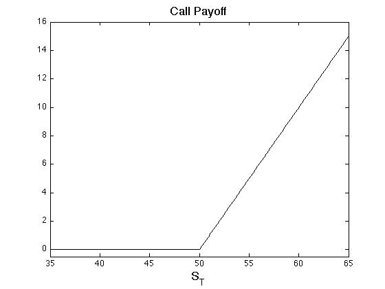
The elementary events [math]\omega_1[/math] and [math]\omega_2[/math] are the two states of the market. The traded assets in this simple market are a bank account, a stock, and and a call option on the stock with exercise at [math]T[/math] and strike [math]K=2[/math]. The market outcomes are shown in Table.

Assets in the Discrete Time-Space Market

time	t=0	t=T
bank account	[math]B_0=1[/math]	[math]B_T=1[/math]\hbox{ (interest rate [math]r=0[/math])}
stock	[math]S_0=2[/math]	[math]S_T = \Big\{\begin{array}{cc}3||\hbox{in }\omega_1 |- |1||\hbox{in }\omega_2\end{array}[/math]
call option, [math]K=2[/math]	[math]C_0=~?[/math]	[math]C_T = \Big\{\begin{array}{cc}1||\hbox{in }\omega_1 |- |0||\hbox{in }\omega_2\end{array}[/math]

The way to determine the price of the call option, [math]C_0[/math], is to replicate it with a portfolio of the stock and the bank account. Let [math]V_t[/math] denote the value of such a portfolio at time [math]t[/math], so that,

[[math]] \begin{eqnarray*} V_0&=&\alpha S_0+\beta\\ V_T&=&\alpha S_T+\beta\ , \end{eqnarray*} [[/math]]

where [math]\alpha[/math] is \# of shares and [math]\beta[/math] is \$ in bank. The portfolio [math]V_t[/math] will replicate the call option if we solve for [math]\alpha[/math] and [math]\beta[/math] so that [math]V_T=C_T[/math] for both [math]\omega_1[/math] and [math]\omega_2[/math],

[[math]] \begin{align*} &3\alpha+\beta=\alpha S_T(\omega_1)+\beta=C_T(\omega_1) =1\\ &\alpha+\beta=\alpha S_T(\omega_1)+\beta=C_T(\omega_2) = 0\ . \end{align*} [[/math]]

This system has solution [math]\alpha = \frac 12[/math], [math]\beta =-\frac 12[/math]. Hence, by the law of one price, it must be that,

[[math]]C_0 = V_0 = \frac 12S_0-\frac 12 = \frac 12. [[/math]]

If [math]C_0\neq V_0[/math], then there would be an arbitrage opportunity in the market. Arbitrage in a financial models means it is possible to purchase a portfolio for which there is a risk-less profit to be earned with positive probability. If such an opportunity is spotted then an investor could borrow an infinite amount of money and buy the arbitrage portfolio, giving him/her an infinite amount of wealth. Arbitrage (in this sense) does not make for a sound financial model, and in real life it is known that true arbitrage opportunities disappear very quickly by the efficiency of the markets. Therefore, almost every financial model assumes absolute efficiency of the market and ‘no-arbitrage’. There is also the concept of ‘No Free Lunch’, but in discrete time-space we do not have to worry about theses differences. The notion of ‘no-arbitrage’ is defined as follows:

Definition

Let [math]wealth_t[/math] denote the wealth of an investor at time [math]t[/math]. We say that the market has arbitrage if,

[[math]] \begin{align*} &\mathbb P(\hbox{wealth}_T \gt 0|\hbox{wealth}_0=0) \gt 0\\ \qquad\hbox{and }\qquad&\mathbb P(\hbox{wealth}_T \lt 0|\hbox{wealth}_0=0)=0\ , \end{align*} [[/math]]

i.e. there is positive probability of a gain and zero probability of a loss.

In our discrete time-space market, if [math]C_0 \lt V_0[/math] then the arbitrage portfolio is one that buys the option, shorts the portfolio, and invest the difference in the bank. The risk-less payoff of this portfolio is shown in Table.

Arbitrage Opportunity if Option Mispriced

	[math]t=0[/math]	[math]t=T[/math]
buy option	[math]-C_0[/math]	[math]\max\{S_T-2,0\}[/math]
sell portfolio	[math]V_0[/math]	[math]-\max\{S_T-2,0\}[/math]
net:	[math]\color{red}{V_0-C_0 \gt 0}[/math]	[math]0[/math]

Equivalent Martingale Measure (EMM)

A common method for pricing an asset is to use a risk-neutral or an equivalent martingale measure (EMM). The EMM is convenient because all asset prices are simply an expectation of the payoff.Two important questions are: what is the EMM? Is there more one?

Definition

The probability measure [math]\mathbb Q[/math] is an EMM of [math]\mathbb P[/math] if [math]S_t[/math] is a [math]\mathbb Q[/math]-martingale, that is

[[math]]\mathbb E^QS_T = S_0[[/math]]

and [math]\mathbb Q[/math] is equivalent to [math]\mathbb P[/math],

[[math]]\mathbb P(\omega) \gt 0\Leftrightarrow \mathbb Q(\omega) \gt 0[[/math]]

for all elementary events [math]\omega\in\Omega[/math] (it's more complicated when [math]\Omega[/math] is not made up of elementary events, but it's basically the same idea).

For our discrete time-space example market, we have

• Under the original measure
  [[math]]\mathbb ES_T = p_1S_T(\omega_1)+p_2S_T(\omega_2)=\frac 23 3+\frac 13 1 = \frac 73 \gt 2=S_0[[/math]]
• Under an EMM [math]\mathbb Q(\omega_1)=q_1[/math] and [math]\mathbb Q(\omega_2)=q_2[/math],
  [[math]] \mathbb E^QS_T=q_13+(1-q_1)1 = 2 = S_0\ .[[/math]]
  Solution is [math]q_1 = \frac 12[/math] and [math]q_2 = 1-q_1 = \frac 12[/math].

Given the EMM, a replicable option is easily priced:

[[math]]\mathbb E^QC_T = \mathbb E^QV_T=\mathbb E^Q[\alpha S_T+\beta]=\alpha\mathbb E^QS_T+\beta =\alpha S_0+\beta = V_0 = C_0\ ,[[/math]]

and so [math]C_0 = \mathbb E^Q\max(S_T-K,2)[/math].

Contingent Claims

A corporation is interested in purchasing a derivative product to provide specific cash-flows for each of the elementary events that (they believe) the market can take. Let [math]\Omega=\{\omega_1,\omega_2,\dots,\omega_N\}[/math] be these elementary events that can occur at time [math]t=T[/math], and let the proposed derivative security be a function [math]C_t(\omega)[/math] such that,

[[math]]C_T(\omega_i) = c_i\qquad\forall i\leq N\ ,[[/math]]

where each [math]c_i[/math] is the corporations desired cash flow. The derivative product [math]C[/math] is a contingent claim, because it pays a fixed amount for all events in the market. Below are some general examples of contingent claims: Example

[[math]](S_T(\omega)-K)^+=\max(S_T(\omega)-K,0)\ ,[[/math]]

where [math]S_T[/math] is some risk asset (e.g. a stock or bond). The payoff on this call option is seen in Figure.

The payoff on a European call option with strike [math]K=50[/math].

Example

[[math]](K-S_T(\omega))^+=\max(K-S_T(\omega),0)\ .[[/math]]

Figure shows the payoff for the put.

The payoff on a European put option with strike [math]K=50[/math].

Example

Example

Example averaged

[[math]]\left(\frac 1M\sum_{\ell=1}^MS_{t_\ell}(\omega)-K\right)^+\ ,[[/math]]

where [math]t_\ell = \ell\frac TM[/math] for integer [math]M \gt 0[/math].

Example

[[math]](S_T^1(\omega)-S_T^2(\omega))^+ ,[[/math]]

where [math]S_t^1[/math] is the price of an asset and [math]S_t^2[/math] is the price of another.

Option Pricing Terminology

The following is a list of terms commonly used in option pricing:

• Long position, a portfolio is ‘long asset X’ if it has net positive holdings of contracts in asset [math]X[/math].
• Short position, a portfolio is ‘short asset X’ if it has net negative holdings of contracts in asset [math]X[/math] (i.e. has short sales of contracts).
• Hedge, or ‘hedging portfolio’ is a portfolio that has minimal or possibly a floor on the losses it might obtain.
• In-the-money (ITM), a derivative contract that would have positive payoff if settlement based on today's market prices (e.g. a call option with very low strike).
• Out-of-the-money (OTM), a derivative contract that would be worthless if settlement based on today's market prices (e.g. a call option with very high strike).
• At-the-money (ATM), a derivative contract exactly at it's breaking point between ITM and OTM.
• Far-from-the-money, a derivative contract with very little chance of finishing ITM.
• Underlying, the stock, bond, ETF, exchange rate, etc. on which a derivative contract is written.
• Strike, The price upon which a call or put option is settled.
• Maturity, the latest time at which a derivative contract can be settled.
• Exercise, the event that the long party decides to use a derivative's embedded option (e.g. using a call option to buy a share of stock at lower than market value).

Completeness \& Fundamental Theorems

The nice thing about the discrete time-space market is that any contingent claim can be replicated. In general, for [math]\Omega=\{\omega_1,\omega_2,\dots,\omega_N\}[/math], and with [math]N-1[/math] risky-assets [math](S^1,S^2,\dots,S^{N-1})[/math] and a risk-free bank account (with [math]r=0[/math]), replicating portfolio weights the contingent claim [math]C[/math] can be found by solving,

[[math]]\begin{pmatrix} 1&S_T^1(\omega_1)&\dots&\dots&S_T^{N-1}(\omega_1)\\ 1&S_T^1(\omega_2)&\dots&\dots&S_T^{N-1}(\omega_2)\\ \vdots&\vdots&\ddots&&\vdots\\ \vdots&\vdots&&\ddots&\vdots\\ 1&S_T^1(\omega_N)&\dots&\dots&S_T^{N-1}(\omega_N) \end{pmatrix} \begin{pmatrix} \beta\\ \alpha_1\\ \vdots\\ \vdots\\ \alpha_{N-1}\\ \end{pmatrix} =\begin{pmatrix} c_1\\ c_2\\ \vdots\\ \vdots\\ c_N \end{pmatrix}\ , [[/math]]

which has a solution [math](\beta,\alpha_1,\dots,\alpha_{N-1})[/math] provided that none of these assets are redundant (e.g., there does not exist a portfolio consisting of the first [math]N-2[/math] assets and the banks account that replicated the [math]S_T^{N-1}[/math]). This [math]N[/math]-dimensional extension of the discrete time-space market serves to further exemplify the importance of replication in asset pricing, and should help to make clear the intentions of the following definition and theorems:

Definition

A contingent claim is reachable if there is a hedging portfolio [math]V[/math] such the [math]V_T(\omega) = C(\omega)[/math] for all [math]\omega[/math], in which case we say that [math]C[/math] can be replicated. If all contingent claims can be replicated, then we say the market is complete. 

Theorem

The 1st fundamental theorem of asset pricing states the market is arbitrage-free if and only if there exists an EMM.

Theorem

The 2nd fundamental theorem of asset pricing states the market is arbitrage-free and complete if and only if there exists a unique EMM.

One of the early works that proves these theorems is . Another good article on the subject is . In summary, these fundamental theorems mean that derivative prices are the expectation under an EMM. ==General references== Papanicolaou, Andrew (2015). "Introduction to Stochastic Differential Equations (SDEs) for Finance". arXiv:1504.05309 [q-fin.MF].

References

- Harrison, M. and Pliska, S. (1981).Martingales and stochastic integrals in the theory of continuous trading.Stochastic Processes and their Applications, (3):215--260.
- Schachermayer, W. (1992).A Hilbert space proof of the fundamental theorem of asset pricing in finite discrete time.Insurance: Mathematics and Economics, 11(4):249--257.