Convolutional Neural Network

[math] require("color") \definecolor{myred}{RGB}{255,77,77} \definecolor{myblue}{RGB}{0,0,255} \definecolor{mygreen}{RGB}{0,230,0} \definecolor{myorange}{RGB}{204, 82, 0} \definecolor{mydarkred}{RGB}{153,0,0} \definecolor{mydarkblue}{RGB}{0,0, 204} \definecolor{mydarkgreen}{RGB}{0,153,0} \definecolor{HeiRot}{RGB}{198,24,38} [/math]

Content for this page was copied verbatim from Herberg, Evelyn (2023). "Lecture Notes: Neural Network Architectures". arXiv:2304.05133 [cs.LG].

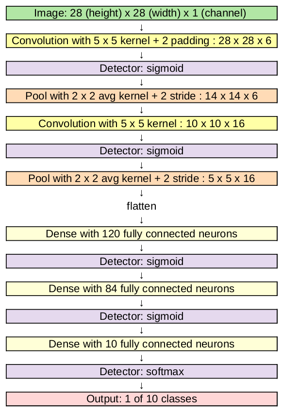
In this section, based on ,, we consider Neural Networks with a different architecture: convolutional neural networks (CNNs or ConvNets). They were first introduced by Kunihiko Fukushima in 1980 under the name "neocognitron" . Famous examples of convolutional neural networks today are "LeNet" , see Figure and "AlexNet" .

As a motivation, consider a classification task where the input is an image of size [math]n_{0,1} \times n_{0,2}[/math] pixels. We want to train a Neural Network so that it can decide, e.g. which digit is written in the image (MNIST data set). We have seen in Figure that the image with [math]n_{0,1}=n_{0,2}=28[/math] has been reshaped (vectorized, flattened) into a vector in [math]\mathbb{R}^{n_{0,1}\cdot n_{0,2}} = \mathbb{R}^{784}[/math], so that we can use it as an input for a regular FNN. However, this approach has several disadvantages:

• Vectorization causes the input image to loose all of its spatial structure, which could have been helpful during training.
• Let e.g. [math]n_{0,1}=n_{0,2}=1000[/math], then [math]n_0 = 10^6[/math] and the weight matrix [math]W^{[0]} \in \mathbb{R}^{n_1 \times 10^6}[/math] contains an enormous number of optimization variables. This can make training very slow or even infeasible.

On the contrary, convolutional neural networks are designed to exploit the relationships between neighboring pixels. In fact, the input of a CNN is typically a matrix or even a three-dimensional tensor, which is then passed through the layers while maintaining this structure. CNNs take small patches, e.g. squares or cubes, from the input images and learn features from them. Consequently, they can subsequently recognize these features in other images, even when they appear in other parts of the image.

Architecture of LeNet-5.

In Figure we see the architecture of "LeNet-5". The inputs are images, where we have 1 channel, because we consider grayscale images. At first we have two sequences of convolution layer (yellow), Section Convolutional Layer , detector layer (violet), Section Detector Layer , and pooling layer (orange), Section Pooling Layer . These layers retain the multidimensional structure of the input. Since this network is built for a classification tasks, the output should be a vector of 10. Consequently, the multi-dimensional output of a hidden layer is flattened, i.e. vectorized, and the remaining layers are fully connected layers (bright yellow) as we have seen in FNNs.

In other, larger architectures, like AlexNet, cf. Figure, to avoid overfitting with large fully connected layers, a technique called dropout is applied. The key idea is to randomly drop units with a given probability and their connections from the neural network during training, for more details we refer to .

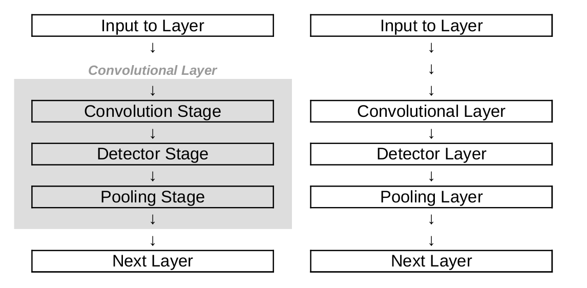
• We will view convolution, detector and pooling layers as separate layers. However, it is also possible to define a convolutional layer to consist of a convolution, detector and pooling stage, cf. Figure. This can be a source of confusion when referring to convolutional layers, which we should be aware of.
• Throughout the remainder of this section we omit layer indices [math]\ell[/math] to simplify notation, and we indicate the data with capital letter [math]Y[/math] to clarify that they are matrices or tensors.

Convolutional layer (gray) consisting of stages (left) compared to viewing the operations as separate layers (right). We use the terminology as depicted on the right hand side, and refer to convolutional, detector and pooling layers as separate layers.

Before we move on to a detailed introduction of the different layer types in CNNs, let us recall the mathematical concept of a convolution.

Convolution

As explained in , in general, convolution describes how one function influences the shape of another function. But it can also be used to apply a weight function to another function, which is how convolution is used in convolutional neural networks.

Definition

Let [math]f, g: \mathbb{R}^n \to \mathbb{R}[/math] be two functions. If both [math]f[/math] and [math]g[/math] are integrable with respect to Lebesgue measure, we can define the convolution as:

[[math]] \begin{align*} c(t) = (f \ast g) (t) = \int f(x) g(t-x) \, dx, \end{align*} [[/math]]

for some [math]t \in \mathbb{R}^n[/math]. Here, [math]f[/math] is called the input and [math]g[/math] is called the kernel. The new function [math]c: \mathbb{R}^n \rightarrow \mathbb{R}[/math] is called the feature map.

However, for convolutional neural networks we need the discrete version.

Definition

Let [math]f, g: \mathbb{Z}^n \to \mathbb{R}[/math] be two discrete functions. The discrete convolution is then defined as:

[[math]] \begin{align*} c(t) = (f \ast g) (t) = \sum_{x \in \mathbb{Z}^n} f(x) g(t - x), \end{align*} [[/math]]

for some [math]t \in \mathbb{Z}^n[/math].

A special case of the discrete convolution is setting [math]f[/math] and [math]g[/math] to [math]n[/math]-dimensional vectors and using the indices as arguments. We illustrate this approach in the following example.

Example

Let [math]X[/math] and [math]Y[/math] be two random variable each describing the outcome of rolling a dice. The probability mass functions are defined as:

[[math]] \begin{align*} f_X(t) = f_Y(t) = \begin{cases} \frac{1}{6}, &\text{if } t \in \{ 1,2,3,4,5,6\}, \\ 0, &\text{if } t \in \mathbb{Z}\setminus\{ 1,2,3,4,5,6\}. \end{cases} \end{align*} [[/math]]

We aim at calculating the probability that the sum of both dice rolls equals nine. To this end, we take the vectors of all possible outcomes and arrange them into two rows. Here, we flip the second vector and slide it to the right, such that the numbers which add to nine align.

Now, we replace the outcomes with their respective probabilities, multiply the adjacent components and add up the results.

This gives

[[math]] f_{X+Y}(9) = \frac{1}{36} + \frac{1}{36} +\frac{1}{36} +\frac{1}{36} = \frac{1}{9}, [[/math]]

i.e. the probability that the sum of the dice equals nine is [math]\frac{1}{9}.[/math] In fact, all the steps we have just done are equivalent to calculating a discrete convolution:

[[math]] \begin{align*} f_{X+Y}(9) = \sum_{x = 1}^6 f_X(x)f_Y(9- x) = (f_X \ast f_Y) (9) \end{align*} [[/math]]

Convolutional Layer

For the convolutional layers in CNNs we define convolutions for matrices, cf. e.g. . This can be extended to tensors straight forward.

Definition

Let [math]Y \in \mathbb{R}^{n_1 \times n_2}[/math] and [math]K \in \mathbb{R}^{m_1 \times m_2}[/math] be given matrices, such that [math]m_1 \leq n_1[/math] and [math]m_2 \leq n_2[/math]. The convolution of [math]Y[/math] and [math]K[/math] is denoted by [math]Y \ast K[/math] with entries

[[math]] \left[ Y \ast K \right]_{i,j} := \sum_{k=1}^{m_1} \sum_{l=1}^{m_2} K_{k,l} Y_{i+m_1-k, j+m_2-l}, [[/math]]

for [math]1 \leq i \leq n_1-m_1 + 1[/math] and [math]1 \leq j \leq n_2 - m_2 +1[/math]. Here, [math]Y[/math] is called the input and [math]K[/math] is called the kernel.

In Machine Learning often the closely related concept of (cross) correlation, cf. e.g. , is used, and incorrectly referred to as convolution, where

[[math]] \left[ Y \circledast K \right]_{i,j} := \sum_{k=1}^{m_1} \sum_{l=1}^{m_2} K_{k,l} Y_{i \color{red}{-1+k}, j \color{red}{-1+l}}, [[/math]]

for [math]1 \leq i \leq n_1-m_1 + 1[/math] and [math]1 \leq j \leq n_2 - m_2 +1[/math]. The (cross) correlation has the same effect as convolution, if you flip both, rows and columns of the kernel [math]K[/math], see the changed indices indicated in red. Since we learn the kernel anyway, it is irrelevant whether the kernel is flipped, thus either concept can be used.

We illustrate the matrix computations with an example.

Example

For this example we have the data matrix

[[math]] \begin{equation*} Y = \begin{pmatrix} 1 & 5 & -2 & 0 & 2 \\ 3 & 8 & 7 & 1 & 0 \\ -1 & 0 & 1 & 2 & 3 \\ 4 & 2 & 1 & -1 & 2 \end{pmatrix}, \end{equation*} [[/math]]

and the kernel

[[math]] \begin{equation*} K = \begin{pmatrix} 1 & 2 & 3 \\ 4 & 5 & 6 \\ 7 & 8 & 9 \end{pmatrix}. \end{equation*} [[/math]]

The computation of [math][Y \ast K]_{1,1}[/math] can be illustrated as follows

[[math]] \begin{equation*} [Y \ast K]_{1,1} = \begin{pmatrix} +1\cdot 9 & +5 \cdot 8 & -2\cdot 7 & \color{gray}{0} & \color{gray}{2} \\ +3 \cdot 6 & +8\cdot 5 & +7\cdot 4 & \color{gray}{1} & \color{gray}{0} \\ -1 \cdot 3 & +0\cdot 2 & +1\cdot 1 & \color{gray}{2} & \color{gray}{3} \\ \color{gray}{4} & \color{gray}{2} & \color{gray}{1} & \color{gray}{-1} & \color{gray}{2} \end{pmatrix} = 9 +40 -14 + 18 +40 +28 - 3 + 0 +1 = 119. \end{equation*} [[/math]]

The gray values of [math]Y[/math] are not used in the computation. Here, we see that [math]K[/math] is flipped when used in the convolution. This also clarifies, how the (cross) correlation can be more intuitive, where

[[math]] \begin{equation*} [Y \circledast K]_{1,1} = \begin{pmatrix} +1\cdot 1 & +5 \cdot 2 & -2\cdot 3 & \color{gray}{0} & \color{gray}{2} \\ +3 \cdot 4 & +8\cdot 5 & +7\cdot 6 & \color{gray}{1} & \color{gray}{0} \\ -1 \cdot 7& +0\cdot 8 & +1\cdot 9 & \color{gray}{2} & \color{gray}{3} \\ \color{gray}{4} & \color{gray}{2} & \color{gray}{1} & \color{gray}{-1} & \color{gray}{2} \end{pmatrix} = 1 + 10 - 6 + 12 +40 + 42 -7 + 0 +9 = 101. \end{equation*} [[/math]]

In a similar way we can proceed to calculate the remaining values by shifting the kernel over the matrix

[[math]] \begin{equation*} [Y \circledast K]_{1,2} = \begin{pmatrix} \color{gray}{1} & +5 \cdot 1 & -2\cdot 2 & +0\cdot 3 & \color{gray}{2} \\ \color{gray}{3} & +8\cdot 4 & +7\cdot 5 & +1 \cdot 6 & \color{gray}{0} \\ \color{gray}{-1} & +0\cdot 7 & +1\cdot 8 & +2 \cdot 9 & \color{gray}{3} \\ \color{gray}{4} & \color{gray}{2} & \color{gray}{1} & \color{gray}{-1} & \color{gray}{2} \end{pmatrix} = 5 -4 + 0 +32 +35 +6 + 0 + 8 +18= 100 . \end{equation*} [[/math]]

Altogether, we get

[[math]] \begin{equation*} Y \ast K = \begin{pmatrix} 119 & 120 & 53 \\ 155 & 155 & 102 \end{pmatrix} \qquad \text{and} \qquad Y \circledast K = \begin{pmatrix} 101 & 100 & 87 \\ 95 & 55 & 58 \end{pmatrix}. \end{equation*} [[/math]]

Especially, [math]Y \ast K \neq Y \circledast K[/math].

An image of size [math]4 \times 5[/math] is divided in blocks of size [math]3 \times 3[/math] by moving one pixel at a time either horizontally or vertically, as shown exemplary in red and green. Here, the black square is denoted by the index [math](1,1)[/math], the red one by [math](1,2)[/math] and the green one by [math](2,1)[/math].

The kernel size, which is typically square, e.g. [math]m \times m[/math], is a hyperparameter of the CNN. Furthermore, the convolutional layer has additional hyperparameters that need to be chosen. We have seen that a convolution with a [math]m \times m[/math] kernel reduces the dimension from [math]n_1\times n_2[/math] to [math]n_1 - m + 1 \times n_2 - m + 1[/math]. To retain the image dimension we can use (zero) padding, cf. , applied to the input [math]Y[/math] with [math]p \in \mathbb{N}_0[/math]. Choosing [math]p=0[/math] yields [math]Y[/math] again, whereas [math]p=1[/math] results in

[[math]] \begin{equation*} \hat Y = \begin{pmatrix} 0 & 0 & 0 & 0 & 0 & 0 & 0\\ 0 & 1 & 5 &-2 & 0 & 2 & 0\\ 0 & 3 & 8 & 7 & 1 & 0 & 0\\ 0 &-1 & 0 & 1 & 2 & 3 & 0 \\ 0 & 4 & 2 & 1 &-1 & 2 & 0 \\ 0 & 0 & 0 & 0 & 0 & 0 & 0 \end{pmatrix}, \end{equation*} [[/math]]

for [math]Y[/math] from Example. Consequently, the padded matrix [math]\hat Y[/math] is of dimension [math](n_1 +2p) \times (n_2+2p) [/math]. To retain the image dimension, we need to choose [math]p[/math] so that

[[math]] \begin{align*} (n_1 + 2p) - m + 1 &= n_1, \\ (n_2 + 2p) - m + 1 &= n_2 , \end{align*} [[/math]]

i.e. [math]p = \frac{m-1}{2}[/math], which is possible for any odd [math]m[/math].

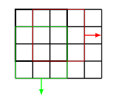
Furthermore, we can choose the stride [math]s\in\mathbb{N}[/math], which indicates how far to move the kernel. For example, in Figure the stride is chosen as [math]s = 1[/math], while the stride in Figure is [math]s=2[/math].

A visualization of the convolution of a [math]7 \times 7[/math] images with a [math]3 \times 3[/math] kernel and stride [math]s=2[/math].

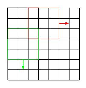
Let us remark that a stride [math]s\gt1[/math] reduces the output dimension of the convolution to

[[math]]\left(\frac{n_1-m}{s}+1\right) \times \left(\frac{n_2-m}{s}+1\right). [[/math]]

Altogether, we can describe the convolutional layer. It consists of [math]M \in \mathbb{N}[/math] filters with identical hyperparameters: kernel size [math]m \times m[/math], padding [math]p[/math] and stride [math]s[/math], but each of them has its own learnable kernel [math]K[/math]. Consequently, the filters in this layer have [math]M\cdot m^2[/math] variables in total. Applying all [math]M[/math] filters to an input matrix [math]Y \in \mathbb{R}^{n_1 \times n_2}[/math] leads to an output of size

[[math]] \left( \frac{n_1 + 2p - m}{s} +1 \right) \times \left( \frac{n_2 + 2p - m}{s} +1 \right) \times M, [[/math]]

where the results for all [math]M[/math] filters are stacked, cf. . Typically, the depth [math]M[/math] is chosen as a power of 2, and growing for deeper layers, while height and width are shrinking, cf. Figure.

Obviously, the output is a tensor with three dimensions, hence the subsequent layers need to process 3-tensor-valued data. In fact, for colored images already the original input of the network is a tensor. The (cross) correlation operation (and also the convolution operation) can be generalized to this case in the following way.

Assume we have an input tensor of size [math] n_1 \times n_2 \times n_3,[/math] then we choose a three dimensional kernel of size

[[math]] m \times m \times n_3 ,[[/math]]

i.e. the depth coincides. No striding or padding is applied in the third dimension. Hence, the output is of dimension

[[math]] \left( \frac{n_1 + 2p - m}{s} +1 \right) \times \left( \frac{n_2 + 2p - m}{s} +1 \right) \times 1, [[/math]]

which can be understood as a matrix by discarding the redundant third dimension, cf. Figure. Doing this for [math]M[/math] filters, again leads to the output being a 3-tensor.

Illustration of a convolution on a tensor, specifically a colored image (with red, green, blue color channels) with a three-dimensional kernel and its result, which is a matrix. Here, no padding [math]p=0[/math] and a single stride [math]s=1[/math] is employed. Image Source: [1].

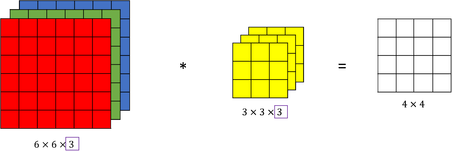
• Convolutional layers have the advantage that they have less variables than fully connected layers applied to the flattened image. For example consider a grayscale image of size [math]28 \times 28[/math] as input in LeNet, cf. Figure. The first convolution has 6 kernels with [math]5\times 5[/math] entries. Due to padding with [math]p=2[/math] the output is [math]28\times 28 \times 6[/math], so the image size is retained. Additionally, before applying a detector layer, we add a bias per channel, so 6 bias variables in this case. In total, we have to learn 156 variables. Now, imagine this image is flattened to a [math]784\times 1[/math] vector and fed into a FNN with fully connected layer, where we also want to retain the size, i.e. the first hidden layer has [math]784[/math] nodes. This results in a much larger number of variables:

  
  

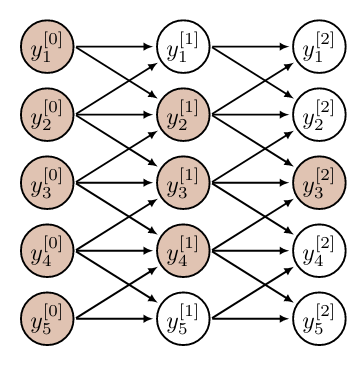
  [[math]] \underbrace{784\cdot784}_{weight}+\underbrace{784}_{bias} = '''615440'''.[[/math]]

• Directly related, a disadvantage of convolutional layers is that every output only sees a subset of all input neurons, cf. e.g. . We denote this set of seen inputs by effective receptive field of the neuron. In an FNN with fully connected layers the effective receptive field of a neuron is the entire input. However, the receptive field of a neuron increases with depth of the network, as illustrated in Figure.

Simplified CNN architecture with an input layer [math]y^{[0]}[/math] and two subsequent convolutional layers [math]y^{[1]}[/math] and [math]y^{[2]}[/math], each with a one dimensional kernel of size [math]m=3[/math], stride [math]s=1[/math] and zero padding [math]p=1[/math]. The colored nodes are the receptive field of the neuron [math]y^{[2]}_3[/math].

Detector Layer

In standard CNN architecture after a convolutional layer, a detector layer is applied. This simply means performing an activation function. To this end, we extend the activation function [math]\sigma:\mathbb{R} \rightarrow \mathbb{R}[/math] to matrix and tensor valued inputs by applying it component-wise, as we did for vectors before in Section Feedforward Neural Network , e.g. for a 3-tensor [math]Y = \{Y_{i,j,k}\}_{i,j,k}[/math] with [math]i=1,\ldots,n_1, j=1,\ldots,n_2, k=1,\ldots,n_3[/math] we get

[[math]] \left(\sigma(Y)\right)_{i,j,k} = \sigma(Y_{i,j,k}). [[/math]]

Pooling Layer

After the detector layer, typically a pooling layer (also called downsampling layer) is applied, cf. e.g. . This layer type is responsible for reducing the first two dimensions (height and width) and usually does not interfere with the third dimension (depth) of the data [math]Y[/math], but rather is applied for all channels independently. Consequently, the depth of the output coincides with the depth of the input and we omit the depth in our discussion.

As in convolutional layers, pooling layers have a filter size [math]m \times m[/math], stride [math]s[/math] and padding [math]p[/math]. However, almost always [math]p=0[/math] is chosen. The most popular values for for the filter size and stride are [math]m=s=2[/math]. Again, with an input of size [math]n_1 \times n_2[/math] the output dimension is

[[math]] \left( \frac{n_1 + 2p -m}{s} +1 \right) \times \left( \frac{n_1 + 2p -m}{s} +1 \right) \quad \stackrel{m=s=2, p=0}{=} \quad \frac{n_1}{2} \times \frac{n_2}{2}. [[/math]]

One common choice is Max Pooling (or Maximum Pooling), where the largest value is selected, cf. e.g. . Below we see an example of max pooling with a [math]2 \times 2[/math] kernel, stride [math]s=2[/math] and no padding.

[[math]] \begin{equation*} \left( \begin{array}{c c | c c} 1 & 3 & 0 & -7 \\ -2 & \color{myorange}{4} & \color{mygreen}{1} & -1 \\ \hline 0 & 1 & \color{HeiRot}{8} & -3 \\ \color{myblue}{2} & 0 & 4 & 5 \end{array} \right) \stackrel{\max}{\longrightarrow} \left( \begin{array}{c | c} \color{myorange}{4} & \color{mygreen}{1} \\ \hline \color{myblue}{2} & \color{HeiRot}{8} \end{array} \right) \end{equation*} [[/math]]

Another common choice is Average Pooling, where we take the mean of all values. Below we see an example of average pooling (abbreviated: "avg") with a [math]2 \times 2[/math] kernel,

[[math]] K = \begin{pmatrix} 0.25 & 0.25 \\ 0.25 & 0.25 \end{pmatrix},[[/math]]

stride [math]s=2[/math] and no padding.

[[math]] \begin{equation*} \hspace{1.2cm} \left( \begin{array}{c c | c c} \color{myorange}{1} & \color{myorange}{3} & \color{mygreen}{0} & \color{mygreen}{-7} \\ \color{myorange}{-2} & \color{myorange}{4} & \color{mygreen}{1} & \color{mygreen}{-1} \\ \hline \color{myblue}{0} & \color{myblue}{1} & \color{HeiRot}{8} & \color{HeiRot}{-3} \\ \color{myblue}{2} & \color{myblue}{0} & \color{HeiRot}{4} & \color{HeiRot}{5} \end{array} \right) \stackrel{\text{avg}}{\longrightarrow} \left( \begin{array}{c | c} \color{myorange}{1.50} & \color{mygreen}{-1.75} \\ \hline \color{myblue}{0.75} & \color{HeiRot}{3.50} \end{array} \right) \end{equation*} [[/math]]

The effect of average pooling applied to an image is easily visible: It blurs the image. In the new image every pixel is an average of a pixel and its neighboring [math]m^2-1[/math] pixels, see Figure. Depending on the choice of stride [math]s[/math] and padding [math]p[/math], the blurred image may also have less pixels.

Original image (left) and blurred image produced by average pooling (right) with a [math]5 \times 5[/math] kernel, stride [math]s=1[/math] and zero padding with [math]p=2[/math]. Image Source: Laurin Ernst.

• Pooling layers do not contain variables to learn.
• We have seen that when using CNNs, we make the following assumptions:
  • Pixels far away from each other do not need to interact with each other.
  • Small translations are not relevant.

Local Response Normalization

Similar to batch normalization, Local Response Normalization (LRN) stabilizes training with unbounded activation functions like ReLU. This strategy was first introduced within the "AlexNet" architecture , cf. Figure, because contrary to previous CNNs like "LeNet-5", which used sigmoid activation, "AlexNet" employs ReLU activation.

Architecture of AlexNet. ReLU activation is employed in the hidden layers. Image Source: [2].

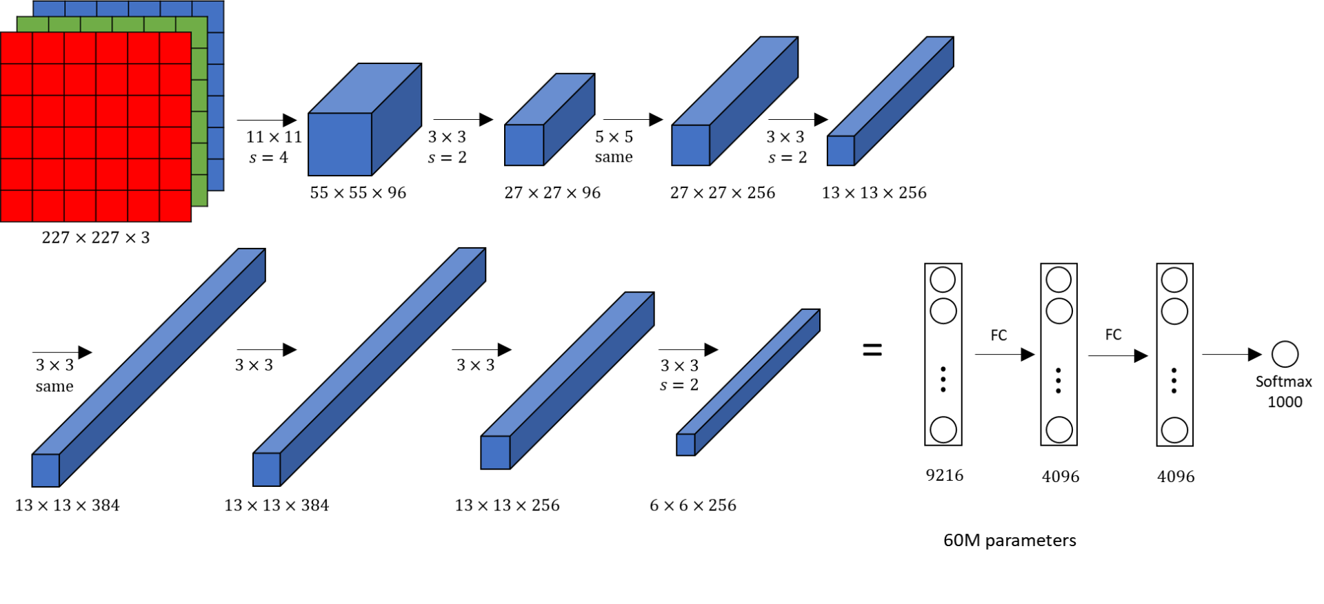
The inter-channel LRN, as introduced in , see also Figure a), is given by

[[math]] \begin{equation*} \hat{Y}_{i,j,k} = \frac{Y_{i,j,k}}{ \left( \kappa + \gamma \sum\limits_{m = \max(1,k-\frac{n}{2})}^{\min(M,k+\frac{n}{2})} (Y_{i,j,m})^2 \right)^\beta }. \end{equation*} [[/math]]

Here, [math]Y_{i,j,k}[/math] and [math]\hat{Y}_{i,j,k}[/math] denote the activity of the neuron before and after normalization, respectively. The indices [math]i,j,k[/math] indicate the height, width and depth of [math]Y[/math]. We have [math]i=1,\ldots,n_1[/math], [math]j=1,\ldots,n_2[/math] and [math]k=1,\ldots,M[/math], where [math]M[/math] is the number of filters in the previous convolutional layer. The values [math]\kappa, \gamma, \beta, n \in \mathbb{R}[/math] are hyperparameters, where [math]\kappa[/math] is used to avoid singularities, and [math]\gamma[/math] and [math]\beta[/math] are called normalization and contrasting constants, respectively. Furthermore, [math]n[/math] dictates how many surrounding neurons are taken into consideration, see also Figure. In [math]\kappa = 2, \gamma = 10^{-4}, \beta = 0.75[/math] were chosen.

Illustration of local response normalization. Inter-channel version a) as introduced in and intra-channel version b). Both for [math]n=2[/math]. For clarification: The red pixel in the top left cube is [math]Y_{1,1,1}[/math], while the red pixel in the top row, second from the left cube is [math]Y_{1,1,2}[/math] and the red pixel in the bottom row, second from the left cube is [math]Y_{1,2,1}[/math]. Image source: [3].

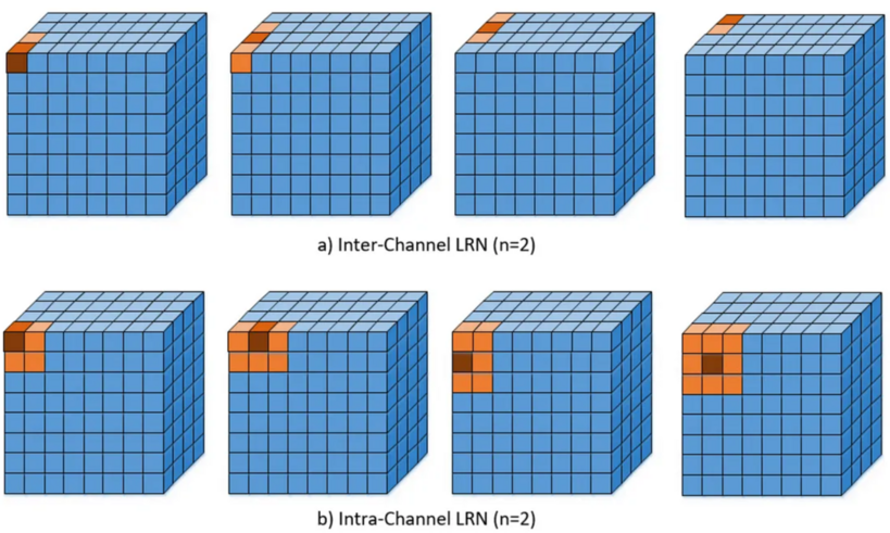
In the case of intra-channel LRN, the neighborhood is extended within the same channel. This leads to the following formula

[[math]] \begin{equation*} \hat{Y}_{i,j,k} = \frac{Y_{i,j,k}}{ \left( \kappa + \gamma \sum\limits_{p = \max(1,i-\frac{n}{2})}^{\min(n_1,i+\frac{n}{2})} \sum\limits_{q = \max(1,j-\frac{n}{2})}^{\min(n_2,j+\frac{n}{2})} (Y_{p,q,k})^2 \right)^\beta }. \end{equation*} [[/math]]

The LRN layer is non-trainable, since it only contains hyperparameters and no variables.

General references

Herberg, Evelyn (2023). "Lecture Notes: Neural Network Architectures". arXiv:2304.05133 [cs.LG].

References

- 1.0 1.1 1.2 1.3 CS231n Convolutional Neural Networks for Visual Recognition, 2023
- 2.0 2.1 2.2 2.3 2.4 2.5 I. Goodfellow, Y. Bengio, and A. Courville. (2016). Deep learning. MIT Press.CS1 maint: multiple names: authors list (link)
- Fukushima, K.. "Neocognitron: A Self-organizing Neural Network Model for a Mechanism of Pattern Recognition Unaffected by Shift in Position". Biological Cybernetics 36.
- Y. LeCun and B. Boser and J. S. Denker and D. Henderson and R. E. Howard and W. Hubbard and L. D. Jackel (1998). "Gradient-based learning applied to document recognition". Proceedings of the IEEE 86.
- 5.0 5.1 5.2 5.3 5.4 5.5 A. Krizhevsky and I. Sutskever and G. E. Hinton (2017). "ImageNet Classification with Deep Convolutional Neural Networks". Communications of the ACM 60.
- Srivastava, N. and Hinton, G. and Krizhevsky, A. and Sutskever, I. and Salakhutdinov, R. (2014). "Dropout: a simple way to prevent neural networks from overfitting". The journal of machine learning research 15. JMLR. org.