Central Limit Theorem for Bernoulli Trials
The second fundamental theorem of probability is the Central Limit Theorem. This theorem says that if [math]S_n[/math] is the sum of [math]n[/math] mutually independent random variables, then the distribution function of [math]S_n[/math] is well-approximated by a certain type of continuous function known as a normal density function, which is given by the formula
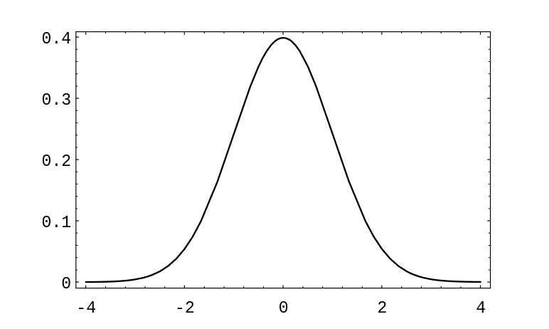
as we have seen in Distributions and Densities . In this section, we will deal only with the case that [math]\mu = 0[/math] and [math]\sigma = 1[/math]. We will call this particular normal density function the x standard normal density, and we will denote it by [math]\phi(x)[/math]:
A graph of this function is given in Figure. It can be shown that the area under any normal density equals 1.
The Central Limit Theorem tells us, quite generally, what happens when we have the sum of a large number of independent random variables each of which contributes a small amount to the total. In this section we shall discuss this theorem as it applies to the Bernoulli trials and in Section \ref{sec 9.3} we shall consider more general processes. We will discuss the theorem in the case that the individual random variables are identically distributed, but the theorem is true, under certain conditions, even if the individual random variables have different distributions.
Bernoulli Trials
Consider a Bernoulli trials process with probability [math]p[/math] for success on each trial. Let [math]X_i = 1[/math] or 0 according as the [math]i[/math]th outcome is a success or failure, and let [math]S_n = X_1 + X_2 +\cdots+ X_n[/math]. Then [math]S_n[/math] is the number of successes in [math]n[/math] trials. We know that [math]S_n[/math] has as its distribution the binomial probabilities [math]b(n,p,j)[/math]. In Combinations, we plotted these distributions for [math]p = .3[/math] and [math]p = .5[/math] for various values of [math]n[/math] (see Figure).
We note that the maximum values of the distributions appeared near the expected
value [math]np[/math], which causes their spike graphs to drift off to the right as
[math]n[/math] increased. Moreover, these maximum values approach 0 as [math]n[/math] increased,
which causes the spike graphs to flatten out.
Standardized Sums
We can prevent the drifting of these spike graphs by subtracting the expected number of successes [math]np[/math] from [math]S_n[/math], obtaining the new random variable [math]S_n - np[/math]. Now the maximum values of the distributions will always be near 0.
To prevent the spreading of these spike graphs, we can normalize [math]S_n - np[/math] to
have variance 1 by dividing by its standard deviation [math]\sqrt{npq}[/math] (see Exercise and Exercise).
The standardized sum of [math]S_n[/math] is given by
Suppose we plot a spike graph with the spikes placed at the possible values of [math]S_n^*[/math]: [math]x_0[/math], [math]x_1[/math], \dots, [math]x_n[/math], where
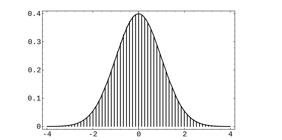
We make the height of the spike at [math]x_j[/math] equal to the distribution value [math]b(n, p, j)[/math]. An example of this standardized spike graph, with [math]n = 270[/math] and [math]p = .3[/math], is shown in Figure. This graph is beautifully bell-shaped. We would like to fit a normal density to this spike graph. The obvious choice to try is the standard normal density, since it is centered at 0, just as the standardized spike graph is. In this figure, we have drawn this standard normal density. The reader will note that a horrible thing has occurred: Even though the shapes of the two graphs are the same, the heights are quite different.
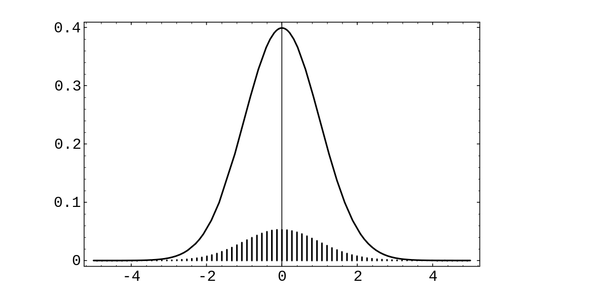
If we want the two graphs to fit each other, we must modify one of them; we choose to modify the
spike graph. Since the shapes of the two graphs look fairly close, we will attempt to modify the
spike graph without changing its shape. The reason for the differing heights is that the sum of
the heights of the spikes equals 1, while the area under the standard normal density equals 1.
If we were to draw a continuous curve through the top of the spikes, and find the area under this
curve, we see that we would obtain, approximately, the sum of the heights of the spikes multiplied
by the distance between consecutive spikes, which we will call [math]\epsilon[/math]. Since the sum of the
heights of the spikes equals one, the area under this curve would be approximately [math]\epsilon[/math].
Thus, to change the spike graph so that the area under this curve has value 1, we need only multiply the heights of the spikes by [math]1/\epsilon[/math]. It is easy to see from Equation \ref{eq 9.1} that
In Figure we show the standardized sum [math]S^*_n[/math] for [math]n = 270[/math] and [math]p = .3[/math], after correcting the heights, together with the standard normal density. (This figure was produced with the program CLTBernoulliPlot.) The reader will note that the standard normal fits the height-corrected spike graph extremely well. In fact, one version of the Central Limit Theorem (see Theorem) says that as [math]n[/math] increases, the standard normal density will do an increasingly better job of approximating the height-corrected spike graphs corresponding to a Bernoulli trials process with [math]n[/math] summands.
Let us fix a value [math]x[/math] on the [math]x[/math]-axis and let [math]n[/math] be a fixed positive integer. Then, using
Equation \ref{eq 9.1}, the point [math]x_j[/math] that is closest to [math]x[/math] has a subscript [math]j[/math] given by the
formula
where [math]\langle a \rangle[/math] means the integer nearest to [math]a[/math]. Thus the height of the spike above [math]x_j[/math] will be
For large [math]n[/math], we have seen that the height of the spike is very close to the height of the normal density at [math]x[/math]. This suggests the following theorem.
(Central Limit Theorem for Binomial Distributions) For the binomial distribution [math]b(n,p,j)[/math] we have
The proof of this theorem can be carried out using Stirling's approximation from
Section \ref{sec 3.1}. We indicate this method of proof by considering the
case [math]x = 0[/math]. In this case, the theorem states that
Approximating Binomial Distributions
We can use Theorem to find approximations for the values of binomial distribution functions. If we wish to find an approximation for [math]b(n, p, j)[/math], we set
and solve for [math]x[/math], obtaining
Theorem then says that
is approximately equal to [math]\phi(x)[/math], so
Example
Let us estimate the probability of exactly 55 heads in 100 tosses of a coin.
For this case [math]np = 100 \cdot 1/2 = 50[/math] and [math]\sqrt{npq} = \sqrt{100 \cdot 1/2
\cdot 1/2} = 5[/math]. Thus [math]x_{55} = (55 - 50)/5 = 1[/math] and
To four decimal places, the actual value is .0485, and so the
approximation is very good.
The program CLTBernoulliLocal illustrates this approximation for any choice of [math]n[/math], [math]p[/math], and [math]j[/math]. We have run this program for two examples. The first is the probability of exactly 50 heads in 100 tosses of a coin; the estimate is .0798, while the actual value, to four decimal places, is .0796. The second example is the probability of exactly eight sixes in 36 rolls of a die; here the estimate is .1093, while the actual value, to four decimal places, is .1196.
The individual binomial probabilities tend to 0 as [math]n[/math] tends to infinity. In
most applications we are not interested in the probability that a specific
outcome occurs, but rather in the probability that the outcome lies in a given
interval, say the interval [math][a, b][/math]. In order to find this probability, we add the
heights of the spike graphs for values of [math]j[/math] between [math]a[/math] and [math]b[/math]. This is the same
as asking for the probability that the standardized sum [math]S_n^*[/math] lies between [math]a^*[/math] and
[math]b^*[/math], where [math]a^*[/math] and [math]b^*[/math] are the standardized values of [math]a[/math] and [math]b[/math]. But as [math]n[/math]
tends to infinity the sum of these areas could be expected to approach the area
under the standard normal density between [math]a^*[/math] and [math]b^*[/math]. The Central Limit Theorem
states that this does indeed happen.
(Central Limit Theorem for Bernoulli Trials) Let [math]S_n[/math] be the number of successes in [math]n[/math] Bernoulli trials with probability [math]p[/math] for success, and let [math]a[/math] and [math]b[/math] be two fixed real numbers. Then
This theorem can be proved by adding together the approximations to [math]b(n,p,k)[/math] given in Theorem. [Notes 1] It is also a special case of the more general Central Limit Theorem (see Section \ref{sec 10.3}).
We know from calculus that the integral on the right side of this equation is
equal to the area under the graph of the standard normal density [math]\phi(x)[/math] between
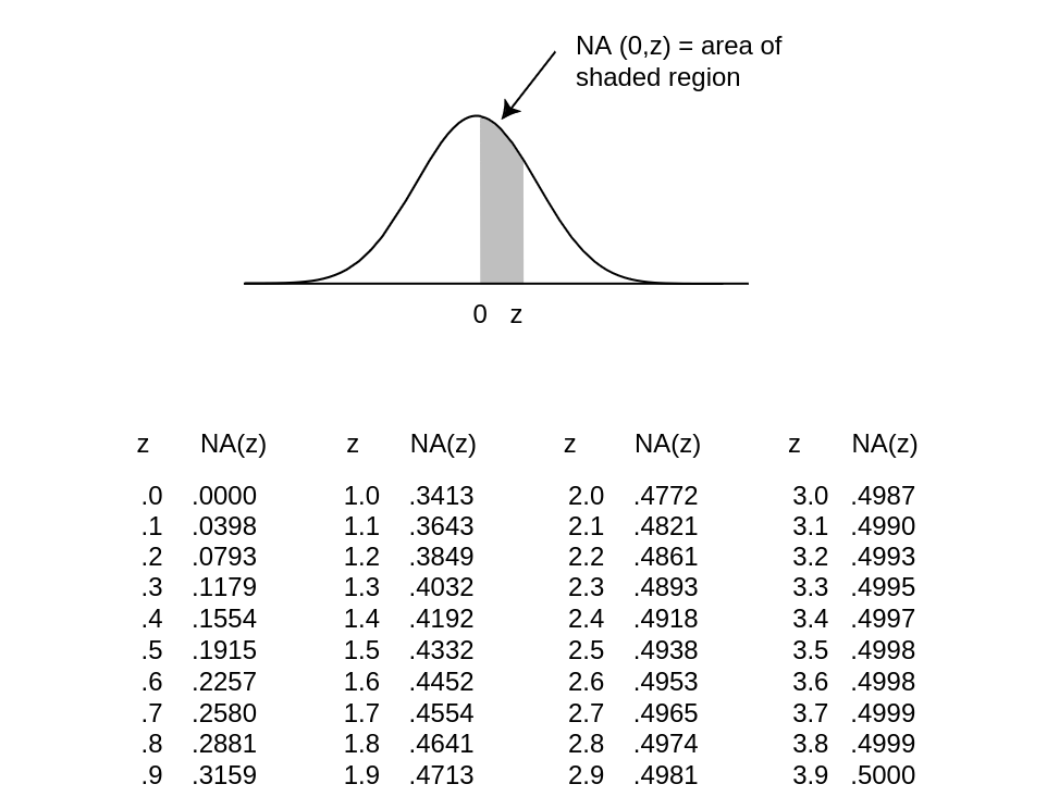
[math]a[/math] and [math]b[/math]. We denote this area by [math]\NA(a^*, b^*)[/math]. Unfortunately, there is no simple way to
integrate the function
[math]e^{-x^2/2}[/math], and so we must either use a table of values or else a numerical
integration program. (See Figure for values of [math]\NA(0, z)[/math]. A more extensive
table is given in Appendix A.)
It is clear from the symmetry of the standard normal density that areas such as that
between [math]-2[/math] and 3 can be found from this table by adding the area from 0 to 2
(same as that from [math]-2[/math] to 0) to the area from 0 to 3.
Approximation of Binomial Probabilities
Suppose that [math]S_n[/math] is binomially distributed with parameters [math]n[/math] and [math]p[/math]. We have seen that the above theorem shows how to estimate a probability of the form
where [math]i[/math] and [math]j[/math] are integers between 0 and [math]n[/math]. As we have seen, the binomial distribution can be represented as a spike graph, with spikes at the integers between 0 and [math]n[/math], and with the height of the [math]k[/math]th spike given by [math]b(n, p, k)[/math]. For moderate-sized values of [math]n[/math], if we standardize this spike graph, and change the heights of its spikes, in the manner described above, the sum of the heights of the spikes is approximated by the area under the standard normal density between [math]i^*[/math] and [math]j^*[/math]. It turns out that a slightly more accurate approximation is afforded by the area under the standard normal density between the standardized values corresponding to [math](i - 1/2)[/math] and [math](j + 1/2)[/math]; these values are
and
Thus,
It should be stressed that the approximations obtained by using the Central Limit Theorem are only approximations, and sometimes they are not very close to the actual values (see Exercise).
We now illustrate this idea with some examples.
Example
A coin is tossed 100 times. Estimate the probability that the number of heads
lies between 40 and 60 (the word “between” in mathematics means inclusive of the endpoints). The
expected number of heads is
[math]100
\cdot 1/2 = 50[/math], and the standard deviation for the number of heads is [math]\sqrt{100 \cdot 1/2
\cdot 1/2} = 5[/math]. Thus, since [math]n = 100[/math] is reasonably large, we have
The actual value is .96480, to five decimal places.
Note that in this case we are asking for the probability that the outcome will
not deviate by more than two standard deviations from the expected value. Had
we asked for the probability that the number of successes is between 35 and 65,
this would have represented three standard deviations from the mean, and, using our 1/2
correction, our estimate would be the area under the standard normal curve between [math]-3.1[/math] and 3.1,
or [math]2\NA(0,3.1) = .9980[/math]. The actual answer in this case, to five places, is .99821.
It is important to work a few problems by hand to understand the conversion from a given inequality to an inequality relating to the standardized variable. After this, one can then use a computer program that carries out this conversion, including the 1/2 correction. The program CLTBernoulliGlobal is such a program for estimating probabilities of the form [math]P(a \leq S_n \leq b)[/math].
Example
Dartmouth College would like to have 1050 freshmen. This college cannot
accommodate more than 1060. Assume that each applicant accepts with
probability .6 and that the acceptances can be modeled by Bernoulli trials.
If the college accepts 1700, what is the probability that it will have too
many acceptances?
If it accepts 1700 students, the expected number of students who matriculate is
[math].6 \cdot 1700 = 1020[/math]. The standard deviation for the number that accept is
[math]\sqrt{1700 \cdot .6 \cdot .4} \approx 20[/math]. Thus we want to estimate the
probability
From Table \ref{tabl 9.1}, if we interpolate, we would estimate this
probability to be [math].5 - .4784 = .0216[/math]. Thus, the college is fairly safe using
this admission policy.
Applications to Statistics
There are many important questions in the field of statistics that can be answered using the Central Limit Theorem for independent trials processes. The following example is one that is encountered quite frequently in the news. Another example of an application of the Central Limit Theorem to statistics is given in Section \ref{sec 9.3}. Example One frequently reads that a poll has been taken to estimate the proportion of people in a certain population who favor one candidate over another in a race with two candidates. (This model also applies to races with more than two candidates [math]A[/math] and [math]B[/math], and two ballot propositions.) Clearly, it is not possible for pollsters to ask everyone for their preference. What is done instead is to pick a subset of the population, called a sample, and ask everyone in the sample for their preference. Let [math]p[/math] be the actual proportion of people in the population who are in favor of candidate [math]A[/math] and let [math]q = 1-p[/math]. If we choose a sample of size [math]n[/math] from the population, the preferences of the people in the sample can be represented by random variables [math]X_1,\ X_2,\ \ldots,\ X_n[/math], where [math]X_i = 1[/math] if person [math]i[/math] is in favor of candidate [math]A[/math], and [math]X_i = 0[/math] if person [math]i[/math] is in favor of candidate [math]B[/math]. Let [math]S_n = X_1 + X_2 + \cdots + X_n[/math]. If each subset of size [math]n[/math] is chosen with the same probability, then [math]S_n[/math] is hypergeometrically distributed. If [math]n[/math] is small relative to the size of the population (which is typically true in practice), then [math]S_n[/math] is approximately binomially distributed, with parameters [math]n[/math] and [math]p[/math].
The pollster wants to estimate the value [math]p[/math]. An estimate for [math]p[/math] is provided by the value
[math]\bar p = S_n/n[/math], which is the proportion of people in the sample who favor candidate [math]B[/math].
The Central Limit Theorem says that the random variable [math]\bar p[/math] is approximately normally
distributed. (In fact, our version of the Central Limit Theorem says that the distribution
function of the random variable
is approximated by the standard normal density.) But we have
i.e., [math]\bar p[/math] is just a linear function of [math]S_n^*[/math]. Since the distribution of [math]S_n^*[/math] is approximated by the standard normal density, the distribution of the random variable [math]\bar p[/math] must also be bell-shaped. We also know how to write the mean and standard deviation of [math]\bar p[/math] in terms of [math]p[/math] and [math]n[/math]. The mean of [math]\bar p[/math] is just [math]p[/math], and the standard deviation is
Thus, it is easy to write down the standardized version of [math]\bar p[/math]; it is
Since the distribution of the standardized version of [math]\bar p[/math] is approximated by the standard normal density, we know, for example, that 95% of its values will lie within two standard deviations of its mean, and the same is true of [math]\bar p[/math]. So we have
Now the pollster does not know [math]p[/math] or [math]q[/math], but he can use [math]\bar p[/math] and [math]\bar q = 1 - \bar p[/math] in their place without too much danger. With this idea in mind, the above statement is equivalent to the statement
The resulting interval
is called the 95 percent confidence interval for the unknown value of [math]p[/math]. The name is suggested by the fact that if we use this method to estimate [math]p[/math] in a large number of samples we should expect that in about 95 percent of the samples the true value of [math]p[/math] is contained in the confidence interval obtained from the sample. In Exercise you are asked to write a program to illustrate that this does indeed happen.
The pollster has control over the value of [math]n[/math]. Thus, if he wants to create a 95% confidence interval with length 6%, then he should choose a value of [math]n[/math] so that
Using the fact that [math]\bar p \bar q \le 1/4[/math], no matter what the value of [math]\bar p[/math] is, it is easy to show that if he chooses a value of [math]n[/math] so that
he will be safe. This is equivalent to choosing
So if the pollster chooses [math]n[/math] to be 1200, say, and calculates [math]\bar p[/math] using his sample of size 1200, then 19 times out of 20 (i.e., 95% of the time), his confidence interval, which is of length 6%, will contain the true value of [math]p[/math]. This type of confidence interval is typically reported in the news as follows: this survey has a 3% margin of error. In fact, most of the surveys that one sees reported in the paper will have sample sizes around 1000. A somewhat surprising fact is that the size of the population has apparently no effect on the sample size needed to obtain a 95% confidence interval for [math]p[/math] with a given margin of error. To see this, note that the value of [math]n[/math] that was needed depended only on the number .03, which is the margin of error. In other words, whether the population is of size 100,00 or 100,00,00, the pollster needs only to choose a sample of size 1200 or so to get the same accuracy of estimate of [math]p[/math]. (We did use the fact that the sample size was small relative to the population size in the statement that [math]S_n[/math] is approximately binomially distributed.)
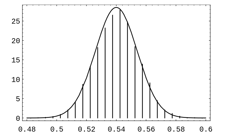
In Figure, we show the results of simulating the polling process. The population
is of size 100,00, and for the population, [math]p = .54[/math]. The sample size was chosen to be
1200. The spike graph shows the distribution of [math]\bar p[/math] for 10,00 randomly chosen
samples. For this simulation, the program kept track of the number of samples for which
[math]\bar p[/math] was within 3% of .54. This number was 9648, which is close to
95% of the number of samples used.
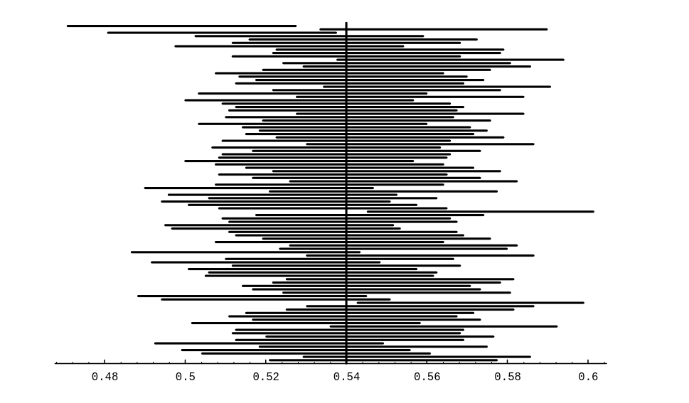
Another way to see what the idea of confidence intervals means is shown in [[#fig
9.2.2|Figure]]. In this figure, we show 100 confidence intervals, obtained by computing [math]\bar p[/math]
for 100 different samples of size 1200 from the same population as before. The reader can see
that most of these confidence intervals (96, to be exact) contain the true value of [math]p[/math].
The Gallup Poll has used these polling techniques in every
Presidential election since 1936 (and in innumerable other
elections as well). Table[Notes 2] shows
the results of their efforts. The reader will note that most of the approximations to [math]p[/math] are
within 3% of the actual value of [math]p[/math]. The sample sizes for these polls were typically around
1500. (In the table, both the predicted and actual percentages for the winning candidate refer
to the percentage of the vote among the “major” political parties. In most elections, there were
two major parties, but in several elections, there were three.)
| Year | [math]\,[/math] Winning | Gallup Final | Election | Deviation |
| Candidate | Survey | Result | ||
| 1936 | Roosevelt | 55.7% | 62.5% | 6.8% |
| 1940 | Roosevelt | 52.0% | 55.0% | 3.0% |
| 1944 | Roosevelt | 51.5% | 53.3% | 1.8% |
| 1948 | Truman | 44.5% | 49.9% | 5.4% |
| 1952 | Eisenhower | 51.0% | 55.4% | 4.4% |
| 1956 | Eisenhower | 59.5% | 57.8% | 1.7% |
| 1960 | Kennedy | 51.0% | 50.1% | 0.9% |
| 1964 | Johnson | 64.0% | 61.3% | 2.7% |
| 1968 | Nixon | 43.0% | 43.5% | 0.5% |
| 1972 | Nixon | 62.0% | 61.8% | 0.2% |
| 1976 | Carter | 48.0% | 50.0% | 2.0% |
| 1980 | Reagan | 47.0% | 50.8% | 3.8% |
| 1984 | Reagan | 59.0% | 59.1% | 0.1% |
| 1988 | Bush | 56.0% | 53.9% | 2.1% |
| 1992 | Clinton | 49.0% | 43.2% | 5.8% |
| 1996 | Clinton | 52.0% | 50.1% | 1.9% |
This technique also plays an important role in the evaluation of the effectiveness of drugs in the
medical profession. For example, it is sometimes desired to know what proportion of patients
will be helped by a new drug. This proportion can be estimated by giving the drug to a subset of
the patients, and determining the proportion of this sample who are helped by the drug.
Historical Remarks
The Central Limit Theorem for Bernoulli trials was first proved by Abraham de Moivre and appeared in his book, The Doctrine of Chances, first published in 1718.[Notes 3] De Moivre spent his years from age 18 to 21 in prison in France because of his Protestant background. When he was released he left France for England, where he worked as a tutor to the sons of noblemen. Newton had presented a copy of his Principia Mathematica to the Earl of Devonshire. The story goes that, while de Moivre was tutoring at the Earl's house, he came upon Newton's work and found that it was beyond him. It is said that he then bought a copy of his own and tore it into separate pages, learning it page by page as he walked around London to his tutoring jobs. De Moivre frequented the coffeehouses in London, where he started his probability work by calculating odds for gamblers. He also met Newton at such a coffeehouse and they became fast friends. De Moivre dedicated his book to Newton. The Doctrine of Chances provides the techniques for solving a wide variety of gambling problems. In the midst of these gambling problems de Moivre rather modestly introduces his proof of the Central Limit Theorem, writing
A Method of approximating the Sum of the Terms of the Binomial [math](a + b)^n[/math] expanded into a Series, from whence are deduced some practical Rules to estimate the Degree of Assent which is to be given to Experiments.[Notes 4]
De Moivre's proof used the approximation to factorials that we now call Stirling's formula. De Moivre states that he had obtained this formula before Stirling but without determining the exact value of the constant [math]\sqrt{2\pi}[/math]. While he says it is not really necessary to know this exact value, he concedes that knowing it “has spread a singular Elegancy on the Solution.”
The complete proof and an interesting discussion of the life of
de Moivre can be found in the book Games, Gods and Gambling by F. N.
David.[Notes 5]
General references
Doyle, Peter G. (2006). "Grinstead and Snell's Introduction to Probability" (PDF). Retrieved June 6, 2024.
Notes
- It is also a special case of the more general Central Limit Theorem. See Section 10.3 of the complete Grinstead-Snell book.
- The Gallup Poll Monthly, November 1992, No.\ 326, p.\ 33. Supplemented with the help of Lydia K. Saab, The Gallup Organization.
- A. de Moivre, The Doctrine of Chances, 3d ed. (London: Millar, 1756).
- ibid., p. 243.
- F. N. David, Games, Gods and Gambling (London: Griffin, 1962).
