Structuring Data without Neural Networks

[math] \newcommand{\varitem}[1]{\vspace{0.1cm}\hspace*{1cm}\raisebox{0.1cm}{ \tikz[baseline=(SebastianoItem.base),remember picture]{% \node[fill=green!20,inner sep=4pt,font=\sffamily] (SebastianoItem){#1};}\hspace{0.25cm} \vspace*{0.1cm}}} \newcommand{\SebastianoHighlight}{\tikz[overlay,remember picture]{% \fill[red!20] ([yshift=-20pt,xshift=-\pgflinewidth]SebastianoItem.east) -- ++(2pt,-2pt) -- ++(-2pt,-2pt) -- cycle; }} \newcommand{\rz}[1]{\displaystyle\stackrel{#1}{\phantom{.}}} % to raise exponent just a bit \newcommand{\CC}{C\nolinebreak\hspace{-.05em}\raisebox{.4ex}{\tiny\bf +}\nolinebreak\hspace{-.10em}\raisebox{.4ex}{\tiny\bf +}} \newcommand{\bm}[1]{\boldsymbol{#1}} \newcommand{\sectionbreak}{\clearpage} \newcommand\pythonstyle{\lstset{ language=Python, basicstyle=\ttm, otherkeywords={self},  % Add keywords here keywordstyle=\ttb\color{deepblue}, emph={MyClass,__init__},  % Custom highlighting emphstyle=\ttb\color{deepred},  % Custom highlighting style stringstyle=\color{deepgreen}, frame=tb,  % Any extra options here showstringspaces=false  % }} \newcommand\pythoninline[1]{{\pythonstyle\lstinline!#1!}} \DeclareMathOperator{\sign}{sign} \newcommand{\mathds}{\mathbb}[/math]

Deep learning with neural networks is very much at the forefront of the recent renaissance in machine learning. However, machine learning is not synonymous with neural networks. There is a wealth of machine learning approaches without neural networks, and the boundary between them and conventional statistical analysis is not always sharp. It is a common misconception that neural network techniques would always outperform these approaches. In fact, in some cases, a simple linear method could achieve faster and better results. Even when we might eventually want to use a deep network, simpler approaches may help to understand the problem we are facing and the specificity of the data so as to better formulate our machine learning strategy. In this chapter, we shall explore machine learning approaches without the use of neural networks. This will further allow us to introduce basic concepts and the general form of a machine learning workflow.

Principle component analysis

At the heart of any machine learning task is data. In order to choose the most appropriate machine learning strategy, it is essential that we understand the data we are working with. However, very often, we are presented with a dataset containing many types of information, called features of the data. Such a dataset is also described as being high-dimensional. Techniques that extract information from such a dataset are broadly summarised as high-dimensional inference. For instance, we could be interested in predicting the progress of diabetes in patients given features such as age, sex, body mass index, or average blood pressure. Extremely high-dimensional data can occur in biology, where we might want to compare gene expression pattern in cells. Given a multitude of features, it is neither easy to visualise the data nor pick out the most relevant information. This is where principle component analysis (PCA) can be helpful. Very briefly, PCA is a systematic way to find out which feature or combination of features varies the most across the data samples. We can think of PCA as approximating the data with a high-dimensional ellipsoid, where the principal axes of this ellipsoid correspond to the principal components. A feature, which is almost constant across the samples, in other words has a very short principal axis, might not be very useful. PCA then has two main applications: (1) It helps to visualise the data in a low dimensional space and (2) it can reduce the dimensionality of the input data to an amount that a more complex algorithm can handle.

PCA algorithm\\ Given a dataset of [math]m[/math] samples with [math]n[/math] data features, we can arrange our data in the form of a [math]m[/math] by [math]n[/math] matrix [math]X[/math] where the element [math]x_{ij}[/math] corresponds to the value of the [math]j[/math]th data feature of the [math]i[/math]th sample. We will also use the feature vector [math]\bm{x}_i[/math] for all the [math]n[/math] features of one sample [math]i=1,\ldots,m[/math]. The vector [math]\bm{x}_i[/math] can take values in the feature space, for example [math]\bm{x}_i \in \mathbb{R}^n[/math]. Going back to our diabetes example, we might have [math]10[/math] data features. Furthermore if we are given information regarding [math]100[/math] patients, our data matrix [math]X[/math] would have [math]100[/math] rows and [math]10[/math] columns. The procedure to perform PCA can then be described as follows:

Principle Component Analysis

• Center the data by subtracting from each column the mean of that column,
  [[math]] \begin{equation} \bm{x}_i \mapsto \bm{x}_{i} - \frac{1}{m} \sum_{i=1}^{m} \bm{x}_{i}. \end{equation} [[/math]]
  This ensures that the mean of each data feature is zero.
• Form the [math]n[/math] by [math]n[/math] (unnormalised) covariance matrix
  [[math]] \begin{equation} C = {X}^{T}{X} = \sum_{i=1}^{m} \bm{x}_{i}\bm{x}_{i}^{T}. \label{eqn: PCA Covariance Matrix} \end{equation} [[/math]]
• Diagonalize the matrix to the form [math]C = {X}^{T}{X} = W\Lambda W^{T}[/math], where the columns of [math]W[/math] are the normalised eigenvectors, or principal components, and [math]\Lambda[/math] is a diagonal matrix containing the eigenvalues. It will be helpful to arrange the eigenvalues from largest to smallest.
• Pick the [math]l[/math] largest eigenvalues [math]\lambda_1, \dots \lambda_l[/math], [math]l\leq n[/math] and their corresponding eigenvectors [math]\bm{v}_1 \dots \bm{v}_l[/math]. Construct the [math]n[/math] by [math]l[/math] matrix [math]\widetilde{W} = [\bm{v}_1 \dots \bm{v}_l][/math].
• Dimensional reduction: Transform the data matrix as
  [[math]] \begin{equation} \label{eqn: PCA Dimensional Reduction} \widetilde{X} = X\widetilde{W}. \end{equation} [[/math]]
  The transformed data matrix [math]\widetilde{X}[/math] now has dimensions [math]m[/math] by [math]l[/math].

We have thus reduced the dimensionality of the data from [math]n[/math] to [math]l[/math]. Notice that there are actually two things happening: First, of course, we now only have [math]l[/math] data features. But second, the [math]l[/math] data features are new features and not simply a selection of the original data. Rather, they are a linear combination of them. Using our diabetes example again, one of the “new” data features could be the sum of the average blood pressure and the body mass index. These new features are automatically extracted by the algorithm. But why did we have to go through such an elaborate procedure to do this instead of simply removing a couple of features? The reason is that we want to maximize the variance in our data. We will give a precise definition of the variance later in the chapter, but briefly the variance just means the spread of the data. Using PCA, we have essentially obtained [math]l[/math] “new” features which maximise the spread of the data when plotted as a function of this feature. We illustrate this with an example.

Example

Let us consider a very simple dataset with just [math]2[/math] data features. We have data, from the Iris dataset, a well known dataset on 3 different species of flowers. We are given information about the petal length and petal width. Since there are just [math]2[/math] features, it is easy to visualise the data. In Fig.fig: Iris PCA, we show how the data is transformed under the PCA algorithm.

PCA on Iris Dataset.

Notice that there is no dimensional reduction here since [math]l = n[/math]. In this case, the PCA algorithm amounts simply to a rotation of the original data. However, it still produces [math]2[/math] new features which are orthogonal linear combinations of the original features: petal length and petal width, i.e.

[[math]] \begin{equation} \begin{split} w_1 &= 0.922 \times \textrm{Petal Length} + 0.388 \times \textrm{Petal Width}, \\ w_2 &= -0.388 \times \textrm{Petal Length} + 0.922 \times \textrm{Petal Width}. \end{split} \end{equation} [[/math]]

We see very clearly that the first new feature [math]w_1[/math] has a much larger variance than the second feature [math]w_2[/math]. In fact, if we are interested in distinguishing the three different species of flowers, as in a classification task, its almost sufficient to use only the data feature with the largest variance, [math]w_1[/math]. This is the essence of (PCA) dimensional reduction. Finally, it is important to note that it is not always true that the feature with the largest variance is the most relevant for the task and it is possible to construct counter examples where the feature with the least variance contains all the useful information. However, PCA is often a good guiding principle and can yield interesting insights in the data. Most importantly, it is also interpretable, i.e., not only does it separate the data, but we also learn which linear combination of features can achieve this. We will see that for many neural network algorithms, in contrast, a lack of interpretability is a big issue.

Kernel PCA

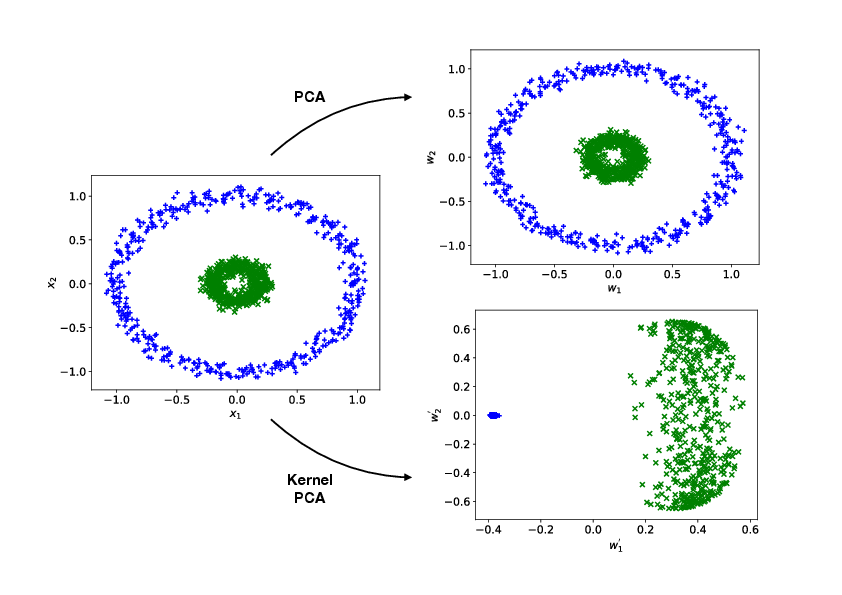
PCA performs a linear transformation on the data. However, there are cases where such a transformation is unable to produce any meaningful result. Consider for instance the fictitious dataset with [math]2[/math] classes and [math]2[/math] data features as shown on the left of Fig.(fig: Kernel PCA). We see by naked eye that it should be possible to separate this data well, for instance by the distance of the datapoint from the origin, but it is also clear that a linear function cannot be used to compute it. In this case, it can be helpful to consider a non-linear extension of PCA, known as kernel PCA. The basic idea of this method is to apply to the data [math]\bm{x} \in \mathbb{R}^{n}[/math] a chosen non-linear vector-valued transformation function [math]\bm{\Phi}(\bm{x})[/math] with

[[math]] \begin{equation}\label{eqn: kernel pca transformation} \bm{\Phi}: \mathbb{R}^{n} \rightarrow \mathbb{R}^{N}, \end{equation} [[/math]]

which is a map from the original [math]n[/math]-dimensional space (corresponding to the [math]n[/math] original data features) to a [math]N[/math]-dimensional feature space. Kernel PCA then simply involves performing the standard PCA on the transformed data [math]\bm{\Phi}(\bm{x})[/math]. Here, we will assume that the transformed data is centered, i.e.,

[[math]] \begin{equation} \sum_i \Phi(\bm{x}_i) = 0 \end{equation} [[/math]]

to have simpler formulas.

Kernel PCA versus PCA.

In practice, when [math]N[/math] is large, it is not efficient or even possible to explicitly perform the transformation [math]\bm{\Phi}[/math]. Instead we can make use of a method known as the kernel trick. Recall that in standard PCA, the primary aim is to find the eigenvectors and eigenvalues of the covariance matrix [math]C[/math]. In the case of kernel PCA, this matrix becomes

[[math]] \begin{equation} C = \sum_{i=1}^{m} \bm{\Phi}(\bm{x}_{i})\bm{\Phi}(\bm{x}_{i})^T, \end{equation} [[/math]]

with the eigenvalue equation

[[math]] \begin{equation} \sum_{i=1}^{m} \bm{\Phi}(\bm{x}_{i})\bm{\Phi}(\bm{x}_{i})^T \bm{v}_{j} = \lambda_{j}\bm{v}_{j}. \label{eqn: pca eigenvalue equation} \end{equation} [[/math]]

By writing the eigenvectors [math]\bm{v}_{j}[/math] as a linear combination of the transformed data features

[[math]] \begin{equation} \bm{v}_{j} = \sum_{i=1}^{m} a_{ji}\bm{\Phi}(\bm{x}_{i}), \end{equation} [[/math]]

we see that finding the eigenvectors is equivalent to finding the coefficients [math]a_{ji}[/math]. On substituting this form back into Eq.\eqref{eqn: pca eigenvalue equation}, we find

[[math]] \begin{equation} \sum_{i=1}^{m} \bm{\Phi}(\bm{x}_{i})\bm{\Phi}(\bm{x}_{i})^T \left[ \sum_{i=1}^{m} a_{ji}\bm{\Phi}(\bm{x}_{j}) \right] = \lambda_{j} \left[ \sum_{i=1}^{m} a_{ji}\bm{\Phi}(\bm{x}_{i}) \right]. \end{equation} [[/math]]

By multiplying both sides of the equation by [math]\bm{\Phi}(\bm{x}_{k})^{T}[/math] we arrive at

[[math]] \begin{equation}\label{eqn: kernel pca eigen equation} \begin{split} \sum_{i=1}^{m} \bm{\Phi}(\bm{x}_{k})^{T} \bm{\Phi}(\bm{x}_{i})\bm{\Phi}(\bm{x}_{i})^T \left[ \sum_{l=1}^{m} a_{jl}\bm{\Phi}(\bm{x}_{l}) \right] &= \lambda_{j} \bm{\Phi}(\bm{x}_{k})^{T} \left[ \sum_{l=1}^{m} a_{jl} \bm{\Phi}(\bm{x}_{l}) \right] \\ \sum_{i=1}^{m} \left[ \bm{\Phi}(\bm{x}_{k})^{T} \bm{\Phi}(\bm{x}_{i}) \right] \sum_{l=1}^{m} a_{jl} \left[ \bm{\Phi}(\bm{x}_{i})^T \bm{\Phi}(\bm{x}_{l}) \right] &= \lambda_{j} \sum_{l=1}^{m} a_{jl} \left[ \bm{\Phi}(\bm{x}_{k})^{T} \bm{\Phi}(\bm{x}_{l}) \right] \\ \sum_{i=1}^{m} K(\bm{x}_{k},\bm{x}_{i}) \sum_{l=1}^{m} a_{jl} K(\bm{x}_{i},\bm{x}_{l}) &= \lambda_{j} \sum_{l=1}^{m} a_{jl} K(\bm{x}_{k},\bm{x}_{l}), \end{split} \end{equation} [[/math]]

where [math]K(\bm{x},\bm{y}) = \bm{\Phi}(\bm{x})^{T} \bm{\Phi}(\bm{y})[/math] is known as the kernel. Thus we see that if we directly specify the kernels we can avoid explicit performing the transformation [math]\bm{\Phi}[/math]. In matrix form, we find the eigenvalue equation [math]K^{2}\bm{a}_{j} = \lambda_{j} K \bm{a}_{j}[/math], which simplifies to

[[math]] \begin{equation} K \bm{a}_{j} = \lambda_{j} \bm{a}_{j}. \end{equation} [[/math]]

Note that this simplification requires [math]\lambda_j \neq 0[/math], which will be the case for relevant principle components. (If [math]\lambda_{j} = 0[/math], then the corresponding eigenvectors would be irrelevant components to be discarded.) After solving the above equation and obtaining the coefficients [math]a_{jl}[/math], the kernel PCA transformation is then simply given by the overlap with the eigenvectors [math]\bm{v}_{j}[/math], i.e.,

[[math]] \begin{equation} \bm{x} \rightarrow \bm{\Phi}(\bm{x}) \rightarrow y_{j} = \bm{v}_{j}^{T}\bm{\Phi}(\bm{x}) = \sum_{i=1}^{m} a_{ji} \bm{\Phi}(\bm{x}_{i})^{T} \bm{\Phi}(\bm{x}) = \sum_{i=1}^{m} a_{ji} K(\bm{x}_{i},\bm{x}), \end{equation} [[/math]]

where once again the explicit [math]\bm{\Phi}[/math] transformation is avoided. A common choice for the kernel is known as the radial basis function kernel (RBF) defined by

[[math]] \begin{equation} K_{\textrm{RBF}}(\bm{x},\bm{y}) = \exp\left( -\gamma \| \bm{x} - \bm{y}\|^{2} \right), \end{equation} [[/math]]

where [math]\gamma[/math] is a tunable parameter. Using the RBF kernel, we compare the result of kernel PCA with that of standard PCA, as shown on the right of Fig.(fig: Kernel PCA). It is clear that kernel PCA leads to a meaningful separation of the data while standard PCA completely fails.

t-SNE as a nonlinear visualization technique

We studied (kernel) PCA as an example for a method that reduces the dimensionality of a dataset and makes features apparent by which data points can be efficiently distinguished. Often, it is desirable to more clearly cluster similar data points and visualize this clustering in a low (two- or three-) dimensional space. We focus our attention on a relatively recent algorithm (from 2008) that has proven very performant. It goes by the name t-distributed stochastic neighborhood embedding (t-SNE). The basic idea is to think of the data (images, for instance) as objects [math]\bm{x}_i[/math] in a very high-dimensional space and characterize their relation by the Euclidean distance [math]||\bm{x}_i-\bm{x}_j||[/math] between them. These pairwise distances are mapped to a probability distribution [math]p_{ij}[/math]. The same is done for the distances [math]||\bm{y}_i-\bm{y}_j||[/math] of the images of the data points [math]\bm{y}_i[/math] in the target low-dimensional space. Their probability distribution is denoted [math]q_{ij}[/math]. The mapping is optimized by changing the locations [math]\bm{y}_i[/math] so as to minimize the distance between the two probability distributions. Let us substantiate these words with formulas. The probability distribution in the space of data points is given as the symmetrized version (joint probability distribution)

[[math]] \begin{equation} p_{ij}=\frac{p_{i|j}+p_{j|i}}{2} \end{equation} [[/math]]

of the conditional probabilities

[[math]] \begin{equation} p_{j|i}=\frac{\mathrm{exp}\left(-||\bm{x}_i-\bm{x}_j||^2/2\sigma_i^2\right)} {\sum_{k\neq i}\mathrm{exp}\left(-||\bm{x}_i-\bm{x}_k||^2/2\sigma_i^2\right)}, \end{equation} [[/math]]

where the choice of variances [math]\sigma_i[/math] will be explained momentarily. Distances are thus turned into a Gaussian distribution. Note that [math]p_{j|i}\neq p_{i|j}[/math] while [math]p_{ji}= p_{ij}[/math]. The probability distribution in the target space is chosen to be a Student t-distribution

[[math]] \begin{equation} q_{ij}=\frac{ (1+||\bm{y}_i-\bm{y}_j||^2)^{-1} }{ \sum_{k\neq l} (1+||\bm{y}_k-\bm{y}_l||^2)^{-1} }. \end{equation} [[/math]]

This choice has several advantages: (i) it is symmetric upon interchanging [math]i[/math] and [math]j[/math], (ii) it is numerically more efficiently evaluated because there are no exponentials, (iii) it has 'fatter' tails which helps to produce more meaningful maps in the lower dimensional space.

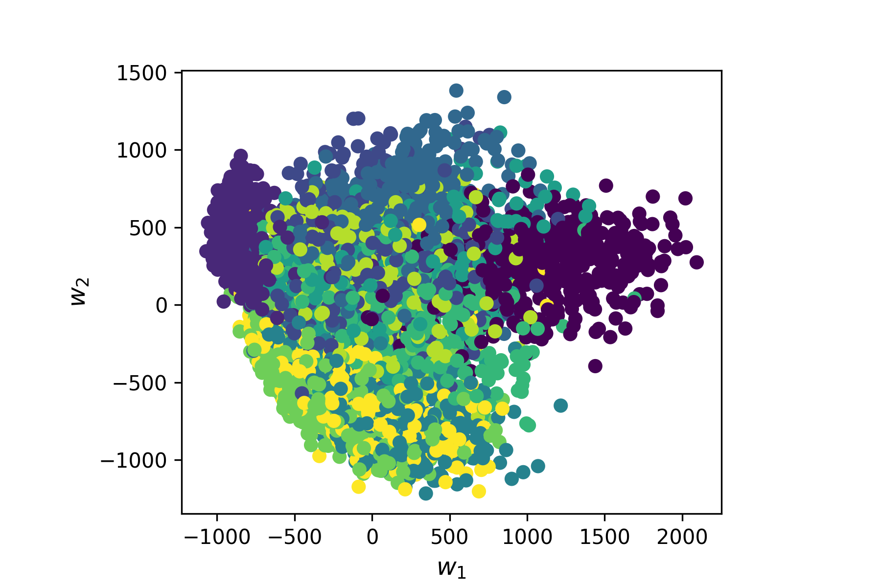
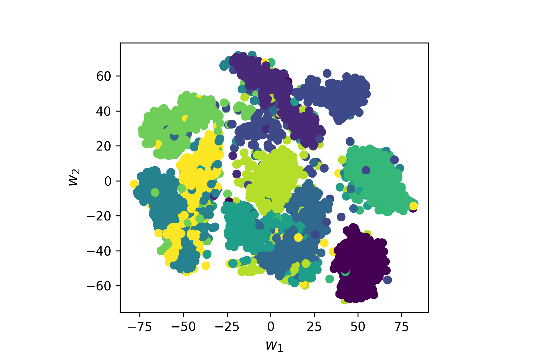
PCA vs.\ t-SNE Application of both methods on 5000 samples from the MNIST handwritten digit dataset. We see that perfect clustering cannot be achieved with either method, but t-SNE delivers the much better result.

Let us now discuss the choice of [math]\sigma_i[/math]. Intuitively, in dense regions of the dataset, a smaller value of [math]\sigma_i[/math] is usually more appropriate than in sparser regions, in order to resolve the distances better. Any particular value of [math]\sigma_i[/math] induces a probability distribution [math]P_i[/math] over all the other data points. This distribution has an entropy (here we use the Shannon entropy, in general it is a measure for the “uncertainty” represented by the distribution)

[[math]] \begin{equation} H(P_i)=-\sum_j p_{j|i}\, \mathrm{log}_2 \,p_{j|i}. \end{equation} [[/math]]

The value of [math]H(P_i)[/math] increases as [math]\sigma_i[/math] increases, i.e., the more uncertainty is added to the distances. The algorithm searches for the [math]\sigma_i[/math] that result in a [math]P_i[/math] with fixed perplexity

[[math]] \begin{equation} \mathrm{Perp}(P_i)=2^{H(P_i)}. \end{equation} [[/math]]

The target value of the perplexity is chosen a priory and is the main parameter that controls the outcome of the t-SNE algorithm. It can be interpreted as a smooth measure for the effective number of neighbors. Typical values for the perplexity are between 5 and 50. Finally, we have to introduce a measure for the similarity between the two probability distributions [math]p_{ij}[/math] and [math]q_{ij}[/math]. This defines a so-called loss function. Here, we choose the Kullback-Leibler divergence

[[math]] \begin{equation} L(\{\bm{y}_i\})=\sum_i\sum_jp_{ij}\mathrm{log}\frac{p_{ij}}{q_{ij}}, \label{eq:KL} \end{equation} [[/math]]

which we will frequently encounter during this lecture. The symmetrized [math]p_{ij}[/math] ensures that [math]\sum_j p_{ij} \gt 1/(2n)[/math], so that each data point makes a significant contribution to the cost function. The minimization of [math]L(\{\bm{y}_i\})[/math] with respect to the positions [math]\bm{y}_i[/math] can be achieved with a variety of methods. In the simplest case it can be gradient descent, which we will discuss in more detail in a later chapter. As the name suggests, it follows the direction of largest gradient of the cost function to find the minimum. To this end it is useful that these gradients can be calculated in a simple form

[[math]] \begin{equation} \frac{\partial L}{\partial \bm{y}_i} =4\sum_j (p_{ij}-q_{ij})(\bm{y}_i-\bm{y}_j)(1+||\bm{y}_i-\bm{y}_j||^2)^{-1}. \end{equation} [[/math]]

By now, t-SNE is implemented as standard in many packages. They involve some extra tweaks that force points [math]\bm{y}_i[/math] to stay close together at the initial steps of the optimization and create a lot of empty space. This facilitates the moving of larger clusters in early stages of the optimization until a globally good arrangement is found. If the dataset is very high-dimensional it is advisable to perform an initial dimensionality reduction (to somewhere between 10 and 100 dimensions, for instance) with PCA before running t-SNE. While t-SNE is a very powerful clustering technique, it has its limitations. (i) The target dimension should be 2 or 3, for much larger dimensions ansatz for [math]q_{ij}[/math] is not suitable. (ii) If the dataset is intrinsically high-dimensional (so that also the PCA pre-processing fails), t-SNE may not be a suitable technique. (iii) Due to the stochastic nature of the optimization, results are not reproducible. The result may end up looking very different when the algorithm is initialized with some slightly different initial values for [math]\bm{y}_i[/math].

Clustering algorithms: the example of [math]k[/math]-means

All of PCA, kernel-PCA and t-SNE may or may not deliver a visualization of the dataset, where clusters emerge. They all leave it to the observer to identify these possible clusters. In this section, we want to introduce an algorithm that actually clusters data, i.e., it will sort any data point into one of [math]k[/math] clusters. Here the desired number of clusters [math]k[/math] is fixed a priori by us. This is a weakness but may be compensated by running the algorithm with different values of [math]k[/math] and asses where the performance is best. We will exemplify a simple clustering algorithm that goes by the name [math]k[/math]-means. The algorithm is iterative. The key idea is that data points are assigned to clusters such that the squared distances between the data points belonging to one cluster and the centroid of the cluster is minimized. The centroid is defined as the arithmetic mean of all data points in a cluster. This description already suggests, that we will again minimize a loss function (or maximize an expectation function, which just differs in the overall sign from the loss function). Suppose we are given an assignment of datapoints [math]\bm{x}_i[/math] to clusters [math]j=1,\cdots, k[/math] that is represented by

[[math]] \begin{equation} w_{ij}=\begin{cases} 1,\qquad \bm{x}_i\text{ in cluster }j,\\ 0,\qquad \bm{x}_i\text{ not in cluster }j. \end{cases} \end{equation} [[/math]]

Then the loss function is given by

[[math]] \begin{equation} L(\{\bm{x}_i\},\{w_{ij}\})=\sum_{i=1}^m\sum_{j=1}^k w_{ij}||\bm{x}_i-\bm{\mu}_j ||^2, \end{equation} [[/math]]

where

[[math]] \begin{equation} \bm{\mu}_j=\frac{\sum_iw_{ij}\bm{x}_i}{\sum_iw_{ij}}. \label{eq: centroids} \end{equation} [[/math]]

Naturally, we want to minimize the loss function with respect to the assignment [math]w_{ij}[/math]. However, a change in this assignment also changes [math]\bm{\mu}_j[/math]. For this reason, it is natural to divide each update step in two parts. The first part updates the [math]w_{ij}[/math] according to

[[math]] \begin{equation} w_{ij}=\begin{cases} 1,\qquad \text{if } j=\mathrm{argmin}_l ||\bm{x}_i-\bm{\mu}_l||,\\ 0,\qquad \text{else }. \end{cases} \end{equation} [[/math]]

That means we attach each data point to the nearest cluster centroid. The second part is a recalculation of the centroids according to Eq.\eqref{eq: centroids}. The algorithm is initialized by choosing at random [math]k[/math] distinct data points as initial positions of the centroids. Then one repeats the above two-part steps until convergence, i.e., until the [math]w_{ij}[/math] do not change anymore. In this algorithm we use the Euclidean distance measure [math]||\cdot ||[/math]. It is advisable to standardize the data such that each feature has mean zero and standard deviation of one when average over all data points. Otherwise (if some features are overall numerically smaller than others), the differences in various features may be weighted very differently by the algorithm. Furthermore, the results depend on the initialization. One should re-run the algorithm with a few different initializations to avoid running into bad local minima. Applications of [math]k[/math]-means are manifold: in economy they include marked segmentation, in science any classification problem such as that of phases of matter, document clustering, image compression (color reduction), etc.. In general it helps to build intuition about the data at hand.

General references

Neupert, Titus; Fischer, Mark H; Greplova, Eliska; Choo, Kenny; Denner, M. Michael (2022). "Introduction to Machine Learning for the Sciences". arXiv:2102.04883 [physics.comp-ph].