Interpretability of Neural Networks

[math] \newcommand{\varitem}[1]{\vspace{0.1cm}\hspace*{1cm}\raisebox{0.1cm}{ \tikz[baseline=(SebastianoItem.base),remember picture]{% \node[fill=green!20,inner sep=4pt,font=\sffamily] (SebastianoItem){#1};}\hspace{0.25cm} \vspace*{0.1cm}}} \newcommand{\SebastianoHighlight}{\tikz[overlay,remember picture]{% \fill[red!20] ([yshift=-20pt,xshift=-\pgflinewidth]SebastianoItem.east) -- ++(2pt,-2pt) -- ++(-2pt,-2pt) -- cycle; }} \newcommand{\rz}[1]{\displaystyle\stackrel{#1}{\phantom{.}}} % to raise exponent just a bit \newcommand{\CC}{C\nolinebreak\hspace{-.05em}\raisebox{.4ex}{\tiny\bf +}\nolinebreak\hspace{-.10em}\raisebox{.4ex}{\tiny\bf +}} \newcommand{\bm}[1]{\boldsymbol{#1}} \newcommand{\sectionbreak}{\clearpage} \newcommand\pythonstyle{\lstset{ language=Python, basicstyle=\ttm, otherkeywords={self},  % Add keywords here keywordstyle=\ttb\color{deepblue}, emph={MyClass,__init__},  % Custom highlighting emphstyle=\ttb\color{deepred},  % Custom highlighting style stringstyle=\color{deepgreen}, frame=tb,  % Any extra options here showstringspaces=false  % }} \newcommand\pythoninline[1]{{\pythonstyle\lstinline!#1!}} \DeclareMathOperator{\sign}{sign} \newcommand{\mathds}{\mathbb}[/math]

In particular for applications in science, we not only want to obtain a neural network that excels at performing a given task, but we also seek an understanding how the problem was solved. Ideally, we want to know underlying principles, deduce causal relations, identify abstracted notions. This is the topic of interpretability.

Dreaming and the problem of extrapolation

Exploring the weights and intermediate activations of a neural network in order to understand what the network has learnt, very quickly becomes unfeasible or uninformative for large network architectures. In this case, we can try a different approach, where we focus on the inputs to the neural network, rather than the intermediate activations.

More precisely, let us consider a neural network classifier [math]\bm{f}[/math], depending on the weights [math]W[/math], which maps an input [math]\bm{x}[/math] to a probability distribution over [math]n[/math] classes [math]\bm{f}(\bm{x}|W) \in \mathbb{R}^{n}[/math], i.e.,

[[math]] \begin{equation} F_{i}(\bm{x}|\theta) \geq 0 \ \ \ \mathrm{and} \ \ \ \sum_{i} F_{i}(\bm{x}|\theta) = 1. \end{equation} [[/math]]

We want to minimise the distance between the output of the network [math]\bm{f(\bm{x})}[/math] and a chosen target output [math]\bm{y}_{\textrm{target}}[/math], which can be done by minimizing the loss function

[[math]] \begin{equation} \label{eqn: dreaming loss} L = |\bm{F}(\bm{x}) - \bm{y}_{\textrm{target}}|^{2}. \end{equation} [[/math]]

However, unlike in supervised learning where the loss minimization was done with respect to the weights [math]W[/math] of the network, here we are interested in minimizing with respect to the input [math]\bm{x}[/math] while keeping the weights [math]W[/math] fixed. This can be achieved using gradient descent, i.e.

[[math]] \begin{equation} \label{eqn: dreaming update} \bm{x} \rightarrow \bm{x} - \eta \frac{\partial L}{\partial \bm{x}}, \end{equation} [[/math]]

where [math]\eta[/math] is the learning rate. With a sufficient number of iterations, our initial input [math]\bm{x}^{0}[/math] will be transformed into the final input [math]\bm{x}^{*}[/math] such that

[[math]] \begin{equation} \bm{f(\bm{x}^*)} \approx \bm{y}_{\textrm{target}}. \end{equation} [[/math]]

By choosing the target output to correspond to a particular class, e.g., [math]\bm{y}_{\textrm{target}} = (1, 0, 0, \dots)[/math], we are then essentially finding examples of inputs which the network would classify as belonging to the chosen class. This procedure is called dreaming.

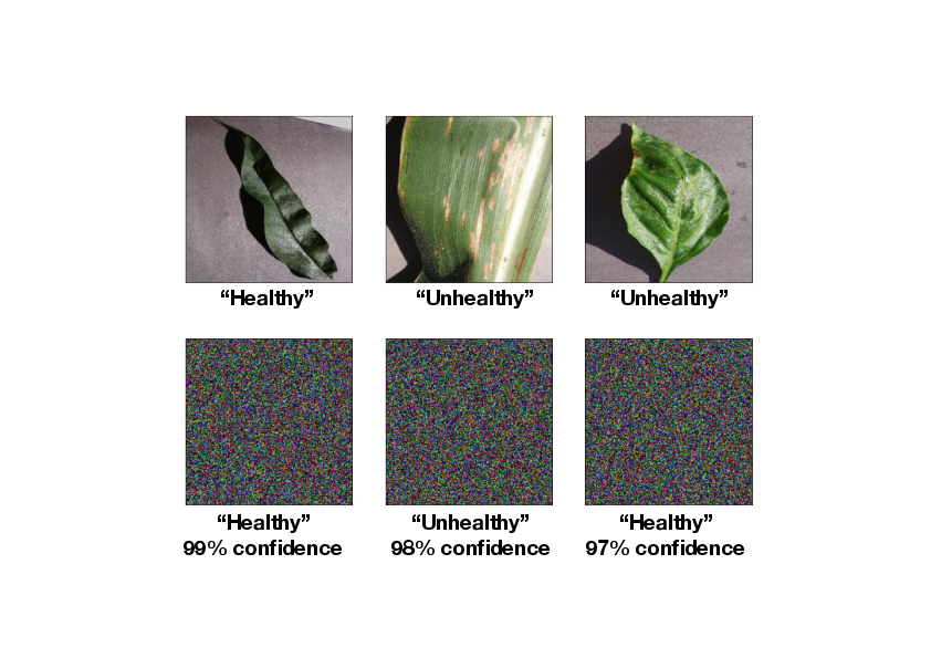
Let us apply this technique to a binary classification example. We consider a dataset consisting of images of healthy and unhealthy plant leaves. Some samples from the dataset are shown in the top row of Fig.fig: dreaming. After training a deep convolutional network to classify the leaves (reaching a test accuracy of around [math]95\%[/math]), we start with a random image as our initial input [math]\bm{x}^{0}[/math] and perform gradient descent on the input, as described above, to arrive at the final image [math]\bm{x}^{*}[/math] which our network confidently classifies.

Plant leaves. Top: Some samples from the plants dataset. Bottom: Samples generated by using the "dreaming" procedure starting from random noise.

In bottom row of Fig.fig: dreaming, we show three examples produced using the ‘dreaming’ technique. On first sight, it might be astonishing that the final image actually does not even remotely resemble a leaf. How could it be that the network has such a high accuracy of around [math]95\%[/math], yet we have here a confidently classified image which is essentially just noise. Although this seem surprising, a closer inspection reveals the problem: The noisy image [math]\bm{x}^{*}[/math] looks nothing like the samples in the dataset with which we trained our network. By feeding this image into our network, we are asking it to make an extrapolation, which as can be seen leads to an uncontrolled behavior. This is a key issue which plagues most data driven machine learning approaches. With few exceptions, it is very difficult to train a model capable of performing reliable extrapolations. Since scientific research is often in the business of making extrapolations, this is an extremely important point of caution to keep in mind. While it might seem obvious that any model should only be predictive for data that ‘resembles’ those in the training set, the precise meaning of ‘resembles’ is actually more subtle than one imagines. For example, if one trains a ML model using a dataset of images captured using a Canon camera but subsequently decide to use the model to make predictions on images taken with a Nikon camera, we could actually be in for a surprise. Even though the images may ‘resemble’ each other to our naked eye, the different cameras can have a different noise profile which might not be perceptible to the human eye. We shall see in the next section that even such minute image distortions can already be sufficient to completely confuse our model.

Adversarial attacks

As we have seen, it is possible to modify the input [math]\bm{x}[/math] so that the corresponding model approximates a chosen target output. This concept can also be applied to generate adverserial examples, i.e. images which have been intentionally modified to cause a model to misclassify it. In addition, we usually want the modification to be minimal or almost imperceptible to the human eye. One common method for generating adversarial examples is known as the fast gradient sign method. Starting from an input [math]\bm{x}^{0}[/math] which our model correctly classifies, we choose a target output [math]\bm{y}^{*}[/math] which corresponds to a wrong classification, and follow the procedure described in the previous section with a slight modification. Instead of updating the input according to Eq.\eqref{eqn: dreaming update} we use the following update rule:

[[math]] \begin{equation} \bm{x} \rightarrow \bm{x} - \eta \ \textrm{sign}\left(\frac{\partial L}{\partial \bm{x}}\right), \end{equation} [[/math]]

where [math]L[/math] is given be Eq.\eqref{eqn: dreaming loss}. The [math]\textrm{sign}(\dots) \in \lbrace -1, 1 \rbrace[/math] both serves to enhance the signal and also acts as constraint to limit the size of the modification. By choosing [math]\eta = \frac{\epsilon}{T}[/math] and performing only [math]T[/math] iterations, we can then guarantee that each component of the final input [math]\bm{x}^{*}[/math] satisfies

[[math]] \begin{equation} |x^{*}_{i} - x^{0}_{i}| \leq \epsilon, \end{equation} [[/math]]

which is important since we want our final image [math]\bm{x}^{*}[/math] to be only minimally modified. We summarize this algorithm as follows:

Fast Gradient Sign Method

Input:

A classification model [math]\bm{f}[/math], a loss function [math]L[/math], an initial image [math]\bm{x}^{0}[/math], a target label [math]\bm{y}_{\textrm{target}}[/math], perturbation size [math]\epsilon[/math] and number of iterations [math]T[/math]

Output:

Adversarial example [math]\bm{x}^{*}[/math] with [math]|x^{*}_{i} - x^{0}_{i}| \leq \epsilon[/math]

[math]\eta = \epsilon/T[/math] ;

for [math]i=1\dots T[/math] do

[math]\bm{x} = \bm{x} - \eta \ \textrm{sign}\left(\frac{\partial L}{\partial \bm{x}}\right)[/math] ;

end

This process of generating adversarial examples is called an adversarial attack, which we can classify under two broad categories: white box and black box attacks. In a white box attack, the attacker has full access to the network [math]\bm{f}[/math] and is thus able to compute or estimate the gradients with respect to the input. On the other hand, in a black box attack, the adversarial examples are generated without using the target network [math]\bm{f}[/math]. In this case, a possible strategy for the attacker is to train his own model [math]\bm{g}[/math], find an adversarial example for his model and use it against his target [math]\bm{f}[/math] without actually having access to it. Although it might seem surprising, this strategy has been found to work albeit with a lower success rate as compared to white box methods. We shall illustrate these concepts in the example below.

Adversarial examples. Generated using the fast gradient sign method with [math]T=1[/math] iteration and [math]\epsilon = 0.01[/math]. The target model is Google's InceptionV3 deep convolutional network with a test accuracy of [math]\sim 95\%[/math] on the binary ("Healthy" vs "Unhealthy") plants dataset.

Example

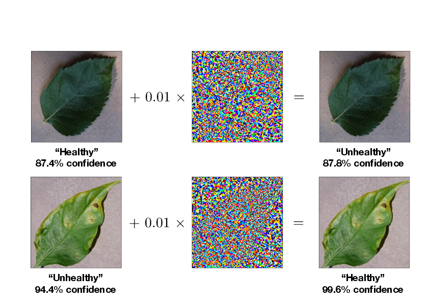
We shall use the same plant leaves classification example as above. The target model [math]\bm{f}[/math] which we want to 'attack' is a pretrained model using Google's well known InceptionV3 deep convolutional neural network containing over [math]20[/math] million parameters. The model achieved a test accuracy of [math]\sim 95\%[/math]. Assuming we have access to the gradients of the model [math]\bm{f}[/math], we can then consider a white box attack. Starting from an image in the dataset which the target model correctly classifies and applying the fast gradient sign method (Alg.\ref{alg: FGSM}) with [math]\epsilon=0.01[/math] and [math]T=1[/math], we obtain an adversarial image which differs from the original image by almost imperceptible amount of noise as depicted on the left of Fig.fig: white box attack. Any human would still correctly identify the image but yet the network, which has around [math]95\%[/math] accuracy has completely failed.

Black Box Adversarial Attack.

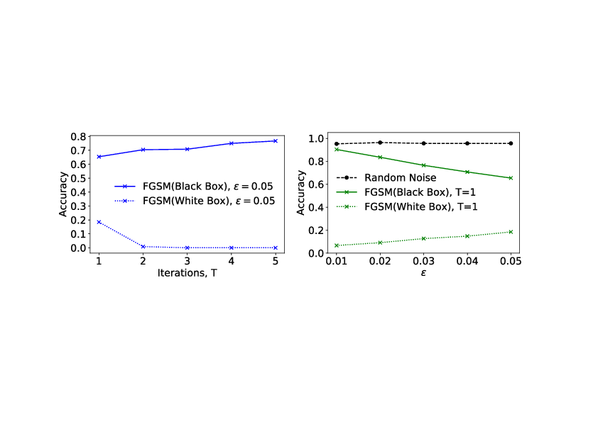
If, however, the gradients and outputs of the target model [math]\bm{f}[/math] are hidden, the above white box attack strategy becomes unfeasible. In this case, we can adopt the following ‘black box attack’ strategy. We train a secondary model [math]\bm{g}[/math], and then applying the FGSM algorithm to [math]\bm{g}[/math] to generate adversarial examples for [math]\bm{g}[/math]. Note that it is not necessary for [math]\bm{g}[/math] to have the same network architecture as the target model [math]\bm{f}[/math]. In fact, it is possible that we do not even know the architecture of our target model. Let us consider another pretrained network based on MobileNet containing about [math]2[/math] million parameters. After retraining the top classification layer of this model to a test accuracy of [math]\sim 95\%[/math], we apply the FGSM algorithm to generate some adversarial examples. If we now test these examples on our target model [math]\bm{f}[/math], we notice a significant drop in the accuracy as shown on the graph on the right of Fig.fig: black box attack. The fact that the drop in accuracy is greater for the black box generated adversarial images as compared to images with random noise (of the same scale) added to it, shows that adversarial images have some degree of transferability between models. As a side note, on the left of Fig.fig: black box attack we observe that black box attacks are more effective when only [math]T=1[/math] iteration of the FGSM algorithm is used, contrary to the situation for the white box attack. This is because, with more iterations, the method has a tendency towards overfitting the secondary model, resulting in adversarial images which are less transferable. These forms of attacks highlight a serious vulnerability of such data driven machine learning techniques. Defending against such attack is an active area of research but it is largely a cat and mouse game between the attacker and defender.

Interpreting autoencoders

Previously we have learned about a broad scope of application of generative models. We have seen that autoencoders can serve as powerful generative models in the scientific context by extracting the compressed representation of the input and using it to generate new instances of the problem. It turns out that in the simple enough problems one can find a meaningful interpretation of the latent representation that may be novel enough to help us get new insight into the problem we are analyzing. In 2020, the group of Renato Renner considered a machine learning perspective on one of the most historically important problems in physics: Copernicus heliocentric system of the solar orbits. Via series of careful and precise measurements of positions of objects in the night sky, Copernicus conjectured that Sun is the center of the solar system and other planets are orbiting around it. Let us now ask the following question: is it possible to build a neural network that receives the same observation angles Copernicus did and deduces the same conclusion from them?

The Copernicus problem. Relation between angles in heliocentric and geocentric coordinate system.

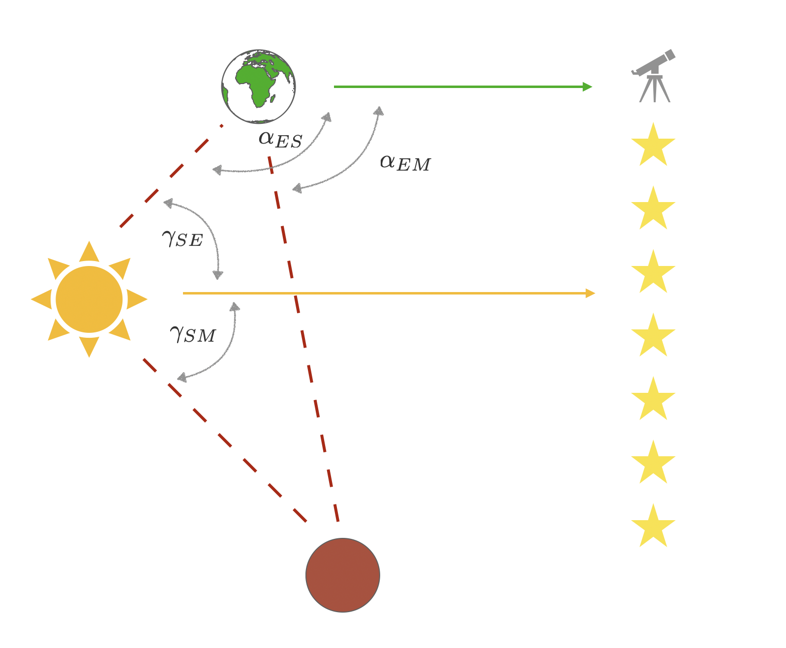
Renner group inputted into the autoencoder the angles of Mars and Sun as observed from Earth ([math]\alpha_{ES}[/math] and [math]\alpha_{EM}[/math] in Fig.fig:copernicus) in certain times and asked the autoencoder to predict the angles at other times. When analyzing the trained model they realized that the two latent neurons included in their model are storing information in the heliocentric coordinates! In particular, one observes that the information stored in the latent space is a linear combination of angles between Sun and Mars, [math]\gamma_{SM}[/math] and Sun and Earth [math]\gamma_{SE}[/math]. In other words, just like Copernicus, the autoencoder has learned, that the most efficient way to store the information given is to transform it into the heliocentric coordinate system.

While this fascinating example is a great way to show the generative models can be interpreted in some important cases, in general the question of interpretability is still very much open and subject to ongoing research. In the instances discussed earlier in this book, like generation of molecules, where the input is compressed through several layers of transformations requiring a complex dictionary and the dimension of the latent space is high, interpreting latent space becomes increasingly challenging.

General references

Neupert, Titus; Fischer, Mark H; Greplova, Eliska; Choo, Kenny; Denner, M. Michael (2022). "Introduction to Machine Learning for the Sciences". arXiv:2102.04883 [physics.comp-ph].