Invariance: Stable Correlations are Causal Correlations

[math] \newcommand{\indep}[0]{\perp\!\!\!\perp} \newcommand{\dpartial}[2]{\frac{\partial #1}{\partial #2}} \newcommand{\abs}[1]{\left| #1 \right|} \newcommand\autoop{\left(} \newcommand\autocp{\right)} \newcommand\autoob{\left[} \newcommand\autocb{\right]} \newcommand{\vecbr}[1]{\langle #1 \rangle} \newcommand{\ui}{\hat{\imath}} \newcommand{\uj}{\hat{\jmath}} \newcommand{\uk}{\hat{k}} \newcommand{\V}{\vec{V}} \newcommand{\half}[1]{\frac{#1}{2}} \newcommand{\recip}[1]{\frac{1}{#1}} \newcommand{\invsqrt}[1]{\recip{\sqrt{#1}}} \newcommand{\halfpi}{\half{\pi}} \newcommand{\windbar}[2]{\Big|_{#1}^{#2}} \newcommand{\rightinfwindbar}[0]{\Big|_{0}^\infty} \newcommand{\leftinfwindbar}[0]{\Big|_{-\infty}^0} \newcommand{\state}[1]{\large\protect\textcircled{\textbf{\small#1}}} \newcommand{\shrule}{\\ \centerline{\rule{13cm}{0.4pt}}} \newcommand{\tbra}[1]{$\bra{#1}$} \newcommand{\tket}[1]{$\ket{#1}$} \newcommand{\tbraket}[2]{$\braket{1}{2}$} \newcommand{\infint}[0]{\int_{-\infty}^{\infty}} \newcommand{\rightinfint}[0]{\int_0^\infty} \newcommand{\leftinfint}[0]{\int_{-\infty}^0} \newcommand{\wavefuncint}[1]{\infint|#1|^2} \newcommand{\ham}[0]{\hat{H}} \newcommand{\mathds}{\mathbb}[/math]

Once we have a probabilistic graphical model, or a structural causal model, that describes the generating process and have a crisp idea of which distribution shifts how, we can come up with a learning algorithm that may alleviate the detrimental effect of such a distribution shift. It is however rare that we can write down the description of a generating process in detail. It is even rarer to have a crisp sense of how distributions shift between training and test times. For instance, how would you describe relationships among millions of pixels of a photo and unobserved identities of objects within it? We can instead focus on devising an alternative way to determine which correlations are considered causal and which other correlations are spurious. The original way to distinguish causal and spurious correlations was entirely reliant on the availability of a full generating process in the form of a probabilistic graphical model. One alternative is to designate correlation that holds both during training and test time as causal, and the rest as spurious. In other words, any correlation that is invariant to the distributional shift is considered causal, while any correlation that varies according to the distributional shift is considered spurious. The goal is then to find a learning algorithm that can ignore spurious (unstable) correlations while capturing only (stable) causal correlations, for the purpose of prediction.

An Environment as a Collider

A case study: a bird or a branch? Imagine a picture of a bird taken from a forest. The bird is probably somewhere near the center of the photo, since the bird is the object of interest. It is extremely difficult to take a good picture of a flying bird, and hence, it is highly likely that the bird is not flying but is sitting. Since we are in a forest, it is highly likely that the bird is sitting on a tree branch with the branch placed near the bottom of the photo. Compare this to a picture with a bird taken from the same forest. the chance of a tree branch being solely near the bottom of the photo is pretty slim. After all, it is a forest, and there are many branches all over. I can then create a bird detector using either of two features; one is a feature describing a bird near the center and the other is a feature describing the location of a tree branch. Clearly, we want our bird detector to use the first feature, that is, to check whether there is a bird in the picture rather than whether there is a tree branch near the bottom of the picture, in order to tell whether there is a bird in the picture. Either way, however, the bird detector would work pretty well in this situation. A bird detector that relies on the position of a tree branch would not work well if suddenly all the pictures are from indoors rather than from a forest. Most of the birds indoors would be confined in their cages and would not be sitting on tree branches. Rather, they would be sitting on an artificial beam or on the ground. On the other hand, a bird detector that relies on the actual appearance features of a bird would continue to work well. That is, the correlation between the label (‘bird’ or not) and the position of a tree branch (‘bottom’ or not) is not stable, while the correlation between the label and the bird-like appearance of a bird is stable. That is, the former is spurious, while the latter is causal. A desirable bird detector would rely on the causal correlation and discard any spurious correlation during learning.

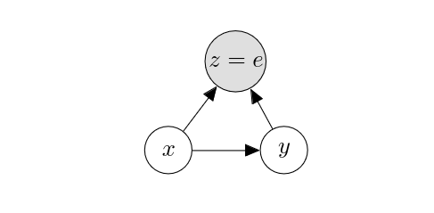
An environment indicator is a collider. A precise mechanism by which these unstable correlations arise can be extremely complex and is often unknown. In other words, we cannot rely on having a precise structural casual model from which we can read out all paths between the input and output, designate each as causal or spurious and adjust for those spurious paths. Instead, we can think of an extremely simplified causal model that includes only three variables; input [math]x[/math], output [math]y[/math] and collider [math]z[/math], as in

In this causal model, the collider [math]z[/math] tell us whether we are in a particular environment (e.g. a forest above.) When we collect data from this causal model while being conditioned on a particular environment, this conditioning on the collider opens the path [math]x \to z \leftarrow y[/math], as we have learned earlier in Confounders, Colliders and Mediators. This way of thinking necessitates a bit of mental contortion. Rather than saying that a particular environment affects the input and output, but we are saying that a particular combination of the input and output probabilistically defines an environment. That is, [math]p(z | x, y)[/math] is the distribution defined over all possible environments [math]z[/math] given the combination of [math]x[/math] and [math]y[/math]. Indeed, if [math]x[/math] is a picture with a tree branch near the bottom of a picture and [math]y[/math] states that there is a bird, the probability of [math]z[/math] being a forest is quite high. The environment dependence can then be thought of as drawing training instances from the graph above where the environment [math]w[/math] takes a particular target environment value (e.g. ‘forest’.) The most naive solution to this issue is to collect as much extra data as possible while avoiding such ‘selection bias’ arising from conditioning the collider [math]z[/math] on any particular value. If we do so, it is as if the collider [math]z[/math] did not exist at all, since marginalizing out [math]z[/math] leads to the following simplified graph:

A predictive model fitted on this graph [math]\hat{p}(y|x)[/math] would capture the causal relationship between the input and output, since the conditional and interventional distributions coincide in this case, that is, [math]p^*(y|x) = p^*(y|\mathrm{do}(x))[/math]. This approach is however often unrealistic.

The Principle of Invariance

Invariant features. So far, we have considered each variable as an unbreakable unit. This is however a very strong assumption, and we should be able to easily split any variable into two or more pieces. This is in fact precisely what we often do by representing an object as a [math]d[/math]-dimensional vector by embedding it into the [math]d[/math]-dimensional Euclidean space. We are splitting a variable [math]x[/math] into a set of [math]d[/math] scalars which collectively representing the value the variable takes. We can then look at a subset of these dimensions and instead of the full variable, in which case the statistical as well as causal relationships with other variables may change. This applies even to a 1-dimensional random variable, where we can apply a nonlinear function to alter its relationship with other variables. Consider the following structural causal model:

[[math]] \begin{align} &x \leftarrow \epsilon_x, \\ &z \leftarrow \mathds{1}(x \gt 0) \max(0, x + \epsilon_z), \\ &y \leftarrow \mathds{1}(x \leq 0) \min(0, x + \epsilon_y) + z , \end{align} [[/math]]

where

[[math]] \begin{align} &\epsilon_x \sim \mathcal{N}(0, 1^2) \\ &\epsilon_z \sim \mathcal{N}(0, 1^2) \\ &\epsilon_y \sim \mathcal{N}(0, 1^2). \end{align} [[/math]]

this model simplifies to [math]y \sim \mathcal{N}(0, 1^2 + 1^2)[/math], where two unit variances come from [math]\epsilon_x[/math] and either [math]\epsilon_z[/math] or [math]\epsilon_y[/math] depending on the sign of [math]x[/math]. With the following nonlinear function applied to [math]x[/math], however, [math]y[/math] takes a different form:

[[math]] \begin{align} g(x) = \mathds{1}(x \leq 0) x. \end{align} [[/math]]

By replacing [math]x[/math] with [math]g(x)[/math] above,

[[math]] \begin{align} p(y) \propto \begin{cases} 0,&\text{ if } y \gt 0, \\ \mathcal{N}(y; 0, 1^2 + 1^2),&\text{ otherwise} \\ \end{cases} \end{align} [[/math]]

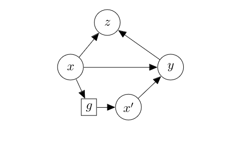
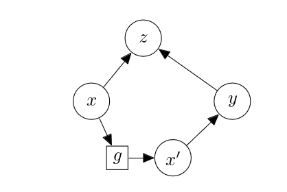
This has the effect of removing the correlation flowing through the path [math]x \to z \to y[/math], leaving only [math]x \to y[/math], because [math]z[/math] is now a constant function regardless of the value [math]x[/math] takes. By inspecting the relationship between [math]g(x)[/math] and [math]y[/math], we can measure the direct causal effect of [math]x[/math] on [math]y[/math]. This example illustrates that there may be a nonlinear function of [math]x[/math] that may results in a variable that preserves enough information to prepare the direct causal relationship between [math]x[/math] and the output [math]y[/math] but removes any relationship [math]x[/math] has with the other variables in the structural causal model. In the context of the environment variable [math]z[/math], which is a collider, the goal is then to find a feature extractor [math]g[/math] such that the original graph is modified into

Ideally, we want [math]g[/math] such that [math]g(x)[/math] explains the whole of [math]x[/math]'s direct effect on [math]y[/math]. That is,

Effectively, [math]x'[/math] works as a mediator between [math]x[/math] and [math]y[/math]. Because [math]g[/math] is a deterministic function, the effect of [math]x[/math] on [math]y[/math] is then perfectly captured by [math]x'[/math]. In order to understand when this would happen, it helps to consider the structural causal model:

[[math]] \begin{align} &x \leftarrow \epsilon_x \\ &x' \leftarrow g(x) \\ &y \leftarrow f_y(x, x', \epsilon_y) \\ &z \leftarrow f_z(x, y, \epsilon_z). \end{align} [[/math]]

What changes between the last two graphs is the third line in the structural causal model above. The original one is

[[math]] \begin{align} y \leftarrow f_y(x, x', \epsilon_y), \end{align} [[/math]]

while the new one is

[[math]] \begin{align} y \leftarrow f'_y(x', \epsilon_y). \end{align} [[/math]]

For this to happen, [math]x'[/math] must absorb all relationship between [math]x[/math] and [math]y[/math]. That is, [math]x'[/math] must be fully predictive of [math]y[/math], leaving only external noise [math]\epsilon_y[/math] and nothing more to be captured by [math]x[/math]. Consider a slightly more realistic example of detecting a fox in a picture. There are two major features of any object within any picture; shape and texture. The shape is what we often want our predictor to rely on, while the texture, which is usually dominated by colour information, should be ignored. For instance, if we have a bunch of pictures taken from any place in the sub-arctic Northern Hemisphere, most of the foxes in these pictures will be yellowish with white-coloured breast and dark-coloured feet and tail. On the other hand, foxes in the pictures taken in the Arctic will largely be white only, implying that the texture/colour feature of a fox is an environment-dependent feature and is not stable across the environments. Meanwhile, the shape information, a fox-like shape, is the invariant feature of a fox across multiple environments. In this case, [math]x'[/math] would be the shape feature of [math]x[/math]. We now see two criteria a function [math]g[/math] must satisfy:

• Given [math]x[/math] and [math]y[/math], [math]x'=g(x)[/math] and [math]z[/math] are independent.
• [math]x'=g(x)[/math] is highly predictive of (correlated with) [math]y[/math].

Once we find such [math]g[/math], the (potentially biased) outcome can be obtained given a new instance [math]x[/math], by fitting a predictive model [math]\hat{p}(y|x')[/math]. That is,

[[math]] \begin{align} \hat{y}(x) = \mathbb{E}_{\hat{p}(y|x'=g(x))} \left[ y \right]. \end{align} [[/math]]

This would be free of the spurious correlation arising from the environment condition.

Learning. We now demonstrate one way to learn [math]g[/math] to satisfy two conditions above as much as possible. First, in order to satisfy the first condition, we must build a predictor of [math]z[/math] given [math]x'[/math]. This predictor should be non-parametric in order to capture as much (higher-order) correlations that could exist between [math]z[/math] and [math]x'[/math]. Let [math]\hat{p}(z|x') = h(x')[/math] be such a predictor obtained by solving the following optimization problem:

[[math]] \begin{align} \label{eq:discriminator-training} \min_{p} -\frac{1}{N} \sum_{n=1}^N \log p(z^n | g(x^n)), \end{align} [[/math]]

where [math](x^n, y^n, z^n)[/math] is the [math]n[/math]-th training example drawn from the original graph while ensuring that [math]z^n \in \mathcal{E}[/math]. [math]\mathcal{E}[/math] is a set of environments in the training set. In other words, we have a few environments we observe and then condition sampling of [math](x,y)[/math] on, and we use these examples to build an environment predictor from [math]g(x)[/math], given [math]g[/math]. The goal is then to minimize the following cost function w.r.t. [math]g[/math], where we assume [math]z[/math] is discrete:

[[math]] \begin{align} C_1(g) = \sum_{z' \in \mathcal{Z}} \hat{p}(z=z'|x'=g(x)) \log \hat{p}(z=z'|x'=g(x)). \end{align} [[/math]]

In other words, we maximize the entropy of [math]\hat{p}(z|x')[/math], which is maximized when it is uniform. When [math]\hat{p}(z|x')[/math] is uniform, it is equivalent to [math]z \indep x'[/math]. One may ask where the condition on observing [math]y[/math] went. This is hidden in [math]\hat{p}(z|x')[/math], since [math]\hat{p}[/math] was estimated using [math](g(x),z)[/math] pairs derived from a set of triples [math](x,y,z)[/math] drawn from the original graph, as clear from Eq.\eqref{eq:discriminator-training}. Of course, this cost function alone is not useful, since it will simply drive [math]g[/math] to be a constant function. The second criterion prevents this, and the second criterion can be expressed as

[[math]] \begin{align} C_2(g, q) = -\frac{1}{N} \sum_{n=1}^N \log q(y^n | g(x^n)). \end{align} [[/math]]

This second criterion must be minimized with respect to both the feature extractor [math]g[/math] and the [math]y[/math] predictor [math]q(y|x')[/math]. This criterion ensures that the feature [math]x'[/math] is predictive of (that is, highly correlated with) the output [math]y[/math]. Given [math]\hat{p}(z|x')[/math], the feature extractor is then trained to minimize

[[math]] \begin{align} \label{eq:feature-training} \min_g C_1(g) + \alpha C_2(g,q), \end{align} [[/math]]

where [math]\alpha[/math] is a hyperparameter and balances between [math]C_1[/math] and [math]C_2[/math]. We then alterate between solving Eq.\eqref{eq:discriminator-training} to find [math]\hat{p}[/math] and solving Eq.\eqref{eq:feature-training} to find [math]g[/math] and [math]\hat{q}[/math]. This is a challenging, bi-level optimization problem and may not even converge both in theory and in practice, although this approach has been used successfully in a few application areas. The most important assumption here is that we have access to training examples from more than one environments. Preferably, we would have examples from all possible environments (that is, from all possible values [math]z[/math] can take), even if they do not necessarily follow [math]p^*(z|x,y)[/math] closely. If so, we would simply ignore [math]z[/math] by considering [math]z[/math] as marginalized. If we have only a small number of environments during training, it will be impossible for us to ensure that [math]g(x)[/math] does not encode any information about [math]z[/math]. There is a connection to generalization, as better generalization in [math]\hat{p}(z|x')[/math] would imply a fewer environments necessary for creating a good [math]\hat{p}(z|x')[/math] and in turn for producing a more stable feature extractor [math]g[/math].

General references

Cho, Kyunghyun (2024). "A Brief Introduction to Causal Inference in Machine Learning". arXiv:2405.08793 [cs.LG].

References

- "Causal inference by using invariant prediction: identification and confidence intervals" (2016). Journal of the Royal Statistical Society Series B: Statistical Methodology 78. Oxford University Press.
- "Invariant risk minimization" (2019). arXiv preprint arXiv:1907.02893.
- "Domain-adversarial training of neural networks" (2016). Journal of machine learning research 17.