Implied Volatility & Local-Volatility Fits

[math] \newcommand{\indicator}[1]{\mathbbm{1}_{\left[ {#1} \right] }} \newcommand{\Real}{\hbox{Re}} \newcommand{\HRule}{\rule{\linewidth}{0.5mm}} \newcommand{\mathds}{\mathbb}[/math]

A major point of discuss with Black-Scholes pricing is the role of volatility. The questions comes about when the Black-Scholes formula is inverted on the market's option prices, which produces an interesting phenomenon known as the implied volatility smile, smirk, or skew. The implied volatility suggests that asset prices are more complex than geometric Brownian motion, and the Black-Scholes' parameter [math]\sigma[/math] needs to be dynamic. Local volatility models and stochastic volatility models are two well-known ways to address this issue; jump-diffusion models and time-change jump models are also a popular choice of model.

Implied Volatility

Implied volatility is the parameter estimate obtained by inverting the Black-Scholes model on market data. The interesting part is that European call and put options will return a different parameter for different strikes and maturity. Let [math]C^{BS}(t,s,k,T,\sigma)[/math] be the Black-Scholes price of a call option with strike [math]K[/math] and maturity [math]T[/math], and let [math]C_t^{data}(K,T)[/math] be the price in the market.

Definition

Implied Volatility is the quantity [math]\hat\sigma(K,T) \gt 0[/math] such that

[[math]]C_t^{data}(K,T) = C^{BS}\left(t,S_t,K,T,\hat\sigma(K,T)\right) \ .[[/math]]

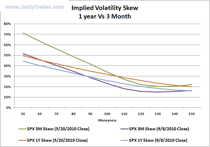
Traders often quote option prices in implied volatility, probably because it is a ‘unit-less’ measure of risk. Typically, the implied smile/skew is plotted as a function of the option's strike as shown in Figure. When plotting implied volatility, the term ‘Moneyness’ refers to how far the option is in-the-money (ITM) or out-of-the-money (OTM). Moneyness can also be interpreted as a unit-less measure, for instance the log-moneyness,

[[math]]\hbox{log-moneyess} = \log(Ke^{-r(T-t)}/S_t)\ .[[/math]]

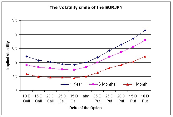
Implied volatility is skewed to the left for many assets, but some assets (such as forex contracts) have a right skew (see Figure). The interpretation is the followoing: implied volatility smile/skew suggests that Black-Scholes is an oversimplification, and the left skew of equity options (such as the SPX ETF options) suggests there is ‘crash-o-phobia’ for long positions in the underlying, and long put options are an insurance item for which there is a premium in the market.\\

Implied Volatility Skew of SPX Index Options. On May 20th, 2010, the S\&P 500 closed at 1072, so moneyness refers to something close to the intrinsic value.

The implied volatility smile for options on the Euro/Yen currency exchange. Notice the skew is to the right.

Bounds on Implied Volatility. There are some bounds on implied volatility that can obtained from the Black-Scholes formula.

Proposition

Changes in implied volatility have bounding inequalities

[[math]]-\frac{e^{-r(T-t)}N(-d_2)}{S_t\sqrt{T-t}N'(d_1)}\leq \frac{\partial}{\partial K}\hat\sigma(K,T)\leq \frac{e^{-r(T-t)}N(d_2)}{S_t\sqrt{T-t}N'(d_1)}[[/math]]

where [math]d_1[/math] and [math]d_2[/math] are given by the Black-Scholes formula and are functions of [math]\hat\sigma[/math].

The derivation of Proposition is as follows:\\ For the call option,

[[math]]\frac{\partial}{\partial K}C_t^{data}(K)=C_k^{BS_1}(t,S_t,K,T,\hat\sigma(K,T))[[/math]]

[[math]]+C_\sigma^{BS}(t,S_t,K,T,\hat\sigma(K,T))\frac{\partial}{\partial K}\hat\sigma(K,T)\leq 0\ ,[[/math]]

hence

[[math]]\frac{\partial}{\partial K}\hat\sigma(K,T)\leq -\frac{C_k^{BS_1}(t,S_t,K,T,\hat\sigma(K,T))}{C_\sigma^{BS}(t,S_t,K,T,\hat\sigma(K,T))}[[/math]]

[[math]] \begin{equation} \label{eq:UB} =\frac{e^{-r(T-t)}N(d_2)}{S_t\sqrt{T-t}N'(d_1)}\ , \end{equation} [[/math]]

where it is straight forward to verify the [math]K[/math]-derivative to be

[[math]]C_k^{BS_1}=\frac{\partial}{\partial K}\left(S_tN(d_1)-Ke^{-r(T-t)}N(d_2)\right) = -N(d_2)\ .[[/math]]

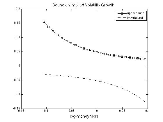
The ratio in \eqref{eq:UB} has the Greek letter vega in the denominator, which causes it to blow-up when [math]K[/math] is far-from-the-money, hence the estimate will be more useful for neat-the-money options (see Figure). A similar inequality is derived from the put option,

[[math]]-\frac{e^{-r(T-t)}N(-d_2)}{S_t\sqrt{T-t}N'(d_1)}\leq \frac{\partial}{\partial K}\hat\sigma(K,T)\ .[[/math]]

This growth bound is also shown in Figure.\\ \bigskip

The growth bound on an option with underlying price [math]S_t = 50[/math], time to maturity [math]T-t=3/13[/math], interest rate [math]r=0[/math], and implied volatility [math]\hat\sigma = .2[/math]. For an ATM option, the bounds of proposition show that derivative of implied volatility with respect to strike to be bounded by about 5%.

Another important bound on implied volatility is the moment formula for options with extreme strike. Let [math]x(K) = \log(Ke^{-r(T-t)}/S_t)[/math]. There exists [math]x^* \gt 0[/math] such that

[[math]] \begin{equation} \label{eq:impVolUB}\hat\sigma(K,T) \lt \sqrt{\frac{2}{T-t}|x(K)|} \end{equation} [[/math]]

for all [math]K[/math] s.t. [math]|x(K)| \gt x^*[/math]. The power of this estimate is that it provides a model-free bound on implied volatility. In other words, it extrapolates the implied volatility smile without assuming any particular structure of the probability distribution. The upper bound in \eqref{eq:impVolUB} can be sharpened to the point where there is uncovered a relationship between implied volatility and the number of finite moments of the underlying [math]S_T[/math].

Proposition (The Moment Formula for Large Strike)

Let

[[math]]\bar p = \sup\{p:\mathbb E^QS_T^{1+p} \lt \infty\}\ ,[[/math]]

and let

[[math]]\beta_R = \lim\sup_{K\rightarrow\infty}\frac{\hat\sigma^2(K,T)}{|x(K)|/T}\ .[[/math]]

Then [math]\beta_R\in[0,2][/math] and

[[math]]\bar p =\frac{1}{2\beta_R}+\frac{\beta_R}{8}-\frac 12\ ,[[/math]]

where [math]1/0\doteq \infty [/math]. Equivalently,

[[math]]\beta_R = 2-4(\sqrt{\bar p^2+\bar p}-\bar p)[[/math]]

where the right-hand side is taken to be zero when [math]\bar p = \infty[/math].

There is also a moment formula for extremely small strikes and [math]\bar q = \sup\{q:\mathbb E^QS_T^{-q} \lt \infty\}[/math]. Both moment formulas are powerful because they are model-free, and because they say that tail behavior of the underlying can be characterized by implied volatility's growth rate against log-moneyness. Indeed, an asset with heavy tails will have higher implied volatility, and so going long or short an option will have more risk, and hence these options will cost more. The important details of the moment formula(s) are in the original paper of Roger Lee .

Local Volatility Function

The idea the volatility is non-constant was first implemented in local volatility models. A local volatility model is a simple extension of Black-Scholes

[[math]]\frac{dS_t}{S_t}=\mu dt+\sigma(t,S_t)dW_t[[/math]]

where the function [math]\sigma(t,s)[/math] is chosen to fit the implied volatility smile. Dependence of [math]\sigma[/math] on [math]S_t[/math] does not effect completeness of market, so there is a pricing PDE that is try similar to the Black-Scholes and is derived in much the same way:

[[math]] \begin{equation} \label{eq:localVolPDE} \left(\frac{\partial}{\partial t}+\frac{S_t^2\sigma^2(t,S_t)}{2}\frac{\partial^2}{\partial s^2} +rS_t\frac{\partial}{\partial s}-r\right)C(t,S_t) = 0 \end{equation} [[/math]]

with terminal condition [math]C\big|_{t=T} = (s-K)^+[/math]. Hence, the Feynmann-Kac formula applies and we have

[[math]]C(t,s) = e^{-r(T-t)}\mathbb E^Q[(S_T-K)^+|S_t=s][[/math]]

where [math]\mathbb E^Q[/math] is a risk-neutral measure under which [math]\frac{dS_t}{S_t} = rdt+\sigma(t,S_t)dW_t^Q[/math]. Now, observe the following facts:

• The first derivative with respect to [math]K[/math] is written with a CDF,
  [[math]] \begin{align*} \frac{\partial}{\partial K}C(t,s) &=e^{-r(T-t)} \frac{\partial}{\partial K}\mathbb E^Q[(S_T-K)^+|S_t= s]\\ &=e^{-r(T-t)} \mathbb E^Q\left[\frac{\partial}{\partial K}(S_T-K)^+\Big|S_t= s\right]\\ &=-e^{-r(T-t)} \mathbb E^Q\left[\indicator{S_T\geq K}\Big|S_t= s\right]\\ &=-e^{-r(T-t)} \mathbb Q(S_T \gt K|S_t=s)\\ &=-e^{-r(T-t)} \left(1 - \mathbb Q(S_T\leq K|S_t=s)\right)\ . \end{align*} [[/math]]
• The second derivative with respect to [math]K[/math] is a PDF,
  [[math]] \begin{align*} \frac{\partial^2}{\partial K^2}C(t,s) &=e^{-r(T-t)} \frac{\partial^2}{\partial K^2}\mathbb E^Q[(S_T-K)^+|S_t= s]\\ &=-e^{-r(T-t)} \frac{\partial}{\partial K}\left(1 - \mathbb Q(S_T\leq K|S_t=s)\right)\\ &=e^{-r(T-t)} \frac{\partial}{\partial K} \mathbb Q(S_T\leq K|S_t=s)\ , \end{align*} [[/math]]
  which is commonly referred to as the Breeden and Litzenberger formula.
• Finally, denote by [math]C(t,s,k)[/math] all the list call options with strike [math]T[/math] and strikes [math]k[/math] ranging from zero to infinity. For a fixed [math]K \gt 0[/math], differentiating with respect to [math]T[/math] and repeated application of integration-by-parts yields the following
  [[math]] \begin{align*} &\frac{\partial}{\partial T}C(t,s,K)\\ =&\frac{\partial}{\partial T}\left(e^{-r(T-t)}\mathbb E^Q[(S_T-K)^+|S_t=s]\right)\\ =&-re^{-r(T-t)}\mathbb E^Q[(S_T-K)^+|S_t=s]+e^{-r(T-t)}\frac{\partial}{\partial T}\mathbb E^Q[(S_T-K)^+|S_t=s]\\ =&-re^{-r(T-t)}\mathbb E^Q\{(S_T-K)^+|S_t=s\}\\ &+e^{-r(T-t)}\frac{\partial}{\partial T}\mathbb E^Q\left[(s-K)^++\int_t^T\left(rS_u\indicator{S_u\geq K}+\frac{\sigma^2(u,S_u)S_u^2}{2}\delta_{K}(S_u)\right)du\Big|S_t=s\right]\\ &+e^{-r(T-t)}\frac{\partial}{\partial T}\underbrace{\mathbb E^Q\left[\int_t^T\sigma(u,S_u)S_u\indicator{S_u\geq K}dW_u^Q\Big|S_t=s\right]}_{=0}\\ =&-re^{-r(T-t)}\mathbb E^Q[(S_T-K)^+|S_t=s]\\ &+e^{-r(T-t)}\mathbb E^Q\left[rS_T\indicator{S_T\geq K}+\frac{\sigma^2(T,S_T)S_T^2}{2}\delta_{K}(S_T)\Big|S_t=s\right]\\ =&rKe^{-r(T-t)}\mathbb E^Q\left[\indicator{S_T\geq K}+\frac{\sigma^2(T,S_T)S_T^2}{2}\delta_{K}(S_T)\Big|S_t=s\right]\\ =&rK\int_0^\infty \indicator{k\geq K}\frac{\partial^2}{\partial k^2}C(t,s,k)dk+\int_0^\infty \frac{\sigma^2(T,k)k^2}{2}\delta_{K}(k)\frac{\partial^2}{\partial k^2}C(t,s,k)dk\\ =&-rK\frac{\partial}{\partial K}C(t,s,K)+ \frac{\sigma^2(T,K)K^2}{2}\frac{\partial^2}{\partial K^2}C(t,s,K)\ .\\ \end{align*} [[/math]]

The above steps 1 through 3 have derived what is known in financial literature as Dupire's Equation:

[[math]] \begin{equation} \label{eq:dupire} \left(\frac{\partial}{\partial T}-\frac{K^2\sigma^2(T,K)}{2}\frac{\partial^2}{\partial K^2}+rK\frac{\partial}{\partial K}\right)C(t,s,K) = 0 \end{equation} [[/math]]

with initial condition [math]C(t,s,K)|_{T=t} = (s-K)^+[/math]. From \eqref{eq:dupire} we get the Dupire scheme for implied local volatility:

[[math]] \begin{equation} \label{eq:dupireFormula} I^2(T,K) = 2\frac{\left(\frac{\partial}{\partial T}+rK\frac{\partial}{\partial K}\right)C }{K^2\frac{\partial^2}{\partial K^2}C} \end{equation} [[/math]]

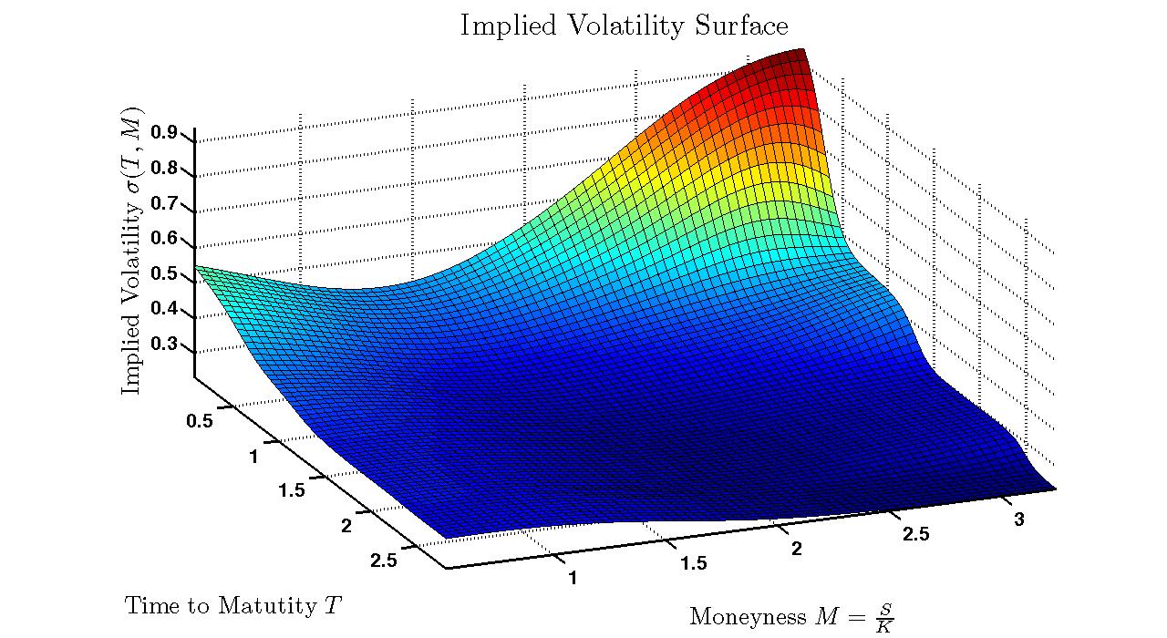
which can be fit to the market's options data for various [math]T[/math]'s and [math]K[/math]'s (see ). This is called ‘calibration of the implied volatility surface’, although methods for calibrating local volatility can be quite complicated with numerical differentiation schemes in [math]T[/math] and [math]K[/math], regularization constraints, etc (for more on fitting techniques see ). Figure shows a calibration of the local volatility surface.\\

Implied Volatility Surface

Shortcomings of Local Volatility. There are some shortcomings of local volatility, one of which is the time dependence or ‘little [math]t[/math]’ effects, which refers to changes in the calibrated surface with time. In other words, the volatility surface will change from day to day, a phenomenon that is inconsistent with [math]\Delta[/math]-hedging arguments for local volatility.

Fitting the Local Volatility Function

Define the log moneyness [math]k=\log(K/S_te^{r(T-t)})[/math], and the time-weighted implied volatility

[[math]] \omega(T,k) = \hat\sigma^2\left(T,S_te^{r(T-t)}e^k\right) (T-t)\ .[[/math]]

It is straight forward to verify that the call-option price can be written with a dimensional version of Black-Scholes formula,

[[math]] \begin{align*} C(t,s,K) &= e^{-r(T-t)}\mathbb E^Q[(S_T-K)^+|S_t=s] \\ &=sC^{BS_1}(\omega(T,k),k)\\ &=s(N(d_1)-e^kN(d_2))\ , \end{align*} [[/math]]

where [math]C^{BS_1}(\omega,k)[/math] is the Black-Scholes call-option price [math]S_t=1[/math], time to maturity [math]T-t=1[/math], strike [math]e^k[/math], interest rate [math]r=0[/math], initial asset price [math]S_t=1[/math], and volatility [math]\sqrt\omega[/math]; the formula parameters are [math]d_1=-k/\sqrt\omega+ \sqrt\omega/2[/math] and [math]d_2=d_1-\sqrt{\omega}[/math]. The dimensionless option price [math]C^{BS_1}(\omega, k)[/math] takes only log moneyness and time-weight volatility, and then the market's option price is proportional to the dimensionless price. Now, there are the following derivatives,

[[math]] \begin{align} \nonumber \frac1s\frac{\partial}{\partial T}C(t,s,K) &= C_k^{BS_1}(\omega(T,k),k)\frac{\partial k}{\partial T}+ C_\omega^{BS_1}(\omega(T,k),k)\frac{\partial \omega(T,k)}{\partial T}\\ \label{eq:dT_C} &=-rC_k^{BS_1}(\omega(T,k),k)+C_\omega^{BS_1}(\omega(T,k),k)\left(\omega_T(T,k)-r\omega_k(T,k)\right)\\ \nonumber &\\ \nonumber \frac1s\frac{\partial}{\partial K}C(t,s,K) &= C_k^{BS_1}(\omega(T,k),k)\frac{\partial k}{\partial K}+C_\omega^{BS_1}(\omega(T,k),k)\frac{\partial \omega(T,k)}{\partial k}\frac{\partial k}{\partial K}\\ \label{eq:dK_C} &=\frac1KC_k^{BS_1}(\omega(T,k),k)+\frac1KC_\omega^{BS}(\omega(T,k),k) \omega_k(T,k)\\ \nonumber &\\ \nonumber \frac1s\frac{\partial^2}{\partial K^2}C(t,s,K) &=\frac{\partial^2}{\partial k^2}C^{BS_1}(\omega(T,k),k)\left(\frac{\partial k}{\partial K}\right)^2+\frac{\partial}{\partial k}C^{BS_1}(\omega(T,k),k)\frac{\partial^2 k}{\partial K^2}\\ \label{eq:dKdK_C} &=\frac{1}{K^2}\left(\frac{\partial^2}{\partial k^2}C^{BS}(\omega(T,k),k)-C_k^{BS_1}(\omega(T,k),k) \right)\ . \end{align} [[/math]]

Plugging \eqref{eq:dT_C}, \eqref{eq:dK_C}, and \eqref{eq:dKdK_C} into the implied local volatility function of \eqref{eq:dupireFormula} yields

[[math]] \begin{align} \label{eq:dupireFormula_impVol_pre} &\sigma^2\left(t,S_te^{r(T-t)}e^k\right) =2 \frac{C_\omega^{BS_1}(\omega(T,k),k) \omega_T(T,k)}{\frac{\partial^2}{\partial k^2}C^{BS_1}(\omega(T,k),k)-\frac{\partial}{\partial k}C^{BS_1}(\omega(T,k),k)}\ . \end{align} [[/math]]

The denominator in \eqref{eq:dupireFormula_impVol_pre} involves the following three derivatives:

[[math]] \begin{align} \label{eq:Cww} C_{\omega\omega}^{BS_1}(\omega,k)&=\left(-\frac18-\frac{1}{2\omega}+\frac{k^2}{2\omega^2}\right)C_\omega^{BS_1}(\omega,k)\\ \label{eq:Cwk} C_{\omega k}^{BS_1}(\omega,k)&=\left(\frac12-\frac k\omega\right)C_\omega^{BS_1}(\omega,k)\\ \label{eq:Ckk-Ck} C_{kk}^{BS_1}(\omega,k)-C_k^{BS_1}(\omega,k)&=2C_\omega^{BS_1}(\omega,k)\ . \end{align} [[/math]]

Using \eqref{eq:Cww}, \eqref{eq:Cwk} and \eqref{eq:Ckk-Ck}, the denominator in \eqref{eq:dupireFormula_impVol_pre} becomes

[[math]] \begin{align*} &\frac{\partial^2}{\partial k^2}C^{BS_1}(\omega(T,k),k)-\frac{\partial}{\partial k}C^{BS_1}(\omega(T,k),k) \\ &=C_{\omega\omega}^{BS_1}(\omega(T,k),k)(\omega_k(T,k))^2+C_\omega^{BS_1}(\omega(T,k),k)w_{kk}(T,k)+2C_{\omega k}^{BS_1}(\omega(T,k),k)\omega_k(T,k)\\ &+C_{kk}^{BS_1}(\omega(T,k),k)-C_\omega^{BS_1}(\omega(T,k),k)\omega_k(T,k)-C_k^{BS_1}(\omega(T,k),k)\\ &=\left\{\left(-\frac18-\frac{1}{2\omega}+\frac{k^2}{2\omega^2}\right)(\omega_k(T,k))^2+w_{kk}(T,k)-\frac{2k}{\omega}\omega_k(T,k)+2\right\}C_\omega^{BS_1}(\omega(T,k),k)\ , \end{align*} [[/math]]

which we then plug into \eqref{eq:dupireFormula_impVol_pre} to get the following implied local volatility formula in terms of the implied volatility surface:

[[math]] \begin{align} \nonumber &\sigma^2\left(T,K\right)\\ \label{eq:dupireFormula_impliedVol} & = \frac{\omega_T(T,k)}{1-\frac{k}{\omega(T,k)}\omega_k(T,k) +\tfrac14\left(-\tfrac14-\tfrac{1}{\omega(T,k)}+\tfrac{k^2}{\omega^2(T,k)}\right)\left(\omega_k(T,k)\right)^2+\frac12\omega_{kk}(T,k)}\ . \end{align} [[/math]]

Surface Parameterizations

Given the formula in \eqref{eq:dupireFormula_impliedVol}, it remains to decide on a differentiable model for [math]\omega(T,k)[/math]. One approach is to find a parametric function [math]f^\theta(T,k)[/math] to fit the implied volatility surface. If the function is once differentiable in [math]T[/math] and twice in [math]k[/math], then the chain rule can be applied to obtain the derivatives in the \eqref{eq:dupireFormula_impliedVol}. Let [math]\theta[/math] be a vector of parameters fit to the weighted surface,

[[math]]\min_\theta\sum_{T,k}\left|f^\theta(T,k)-\omega(T,k)\right| \ ,[[/math]]

where [math]f^\theta[/math] is the parametric function. Given a fit [math]\theta[/math], we need to check that

• the fitted surface is a free from calendar-spread arbitrage,
• and each time slice is free of butterfly arbitrage.

Proposition

The fitted surface is free from calendar-spread arbitrage if

[[math]]f_T^\theta(T,k) \geq 0\ ;[[/math]]

in other words the slices of the weighted surface cannot intersect.

To prevent butterfly arbitrage, effectively we need to ensure that the option price yields a probability density function,

[[math]]\frac{d}{dK}\mathbb P^Q(S_T\leq K|\mathcal F_t) = e^{r(T-t)}\frac{\partial^2}{\partial K^2}C(t,T,K) \ .[[/math]]

Using the parameterized surface, this density is

[[math]] \begin{align*} e^{r(T-t)}\frac{\partial^2}{\partial k^2}C(t,T,K)&= se^{r(T-t)}\frac{\partial^2}{\partial k^2}C^{BS_1}(f^\theta(T,k),k)\\ &=\frac{g^\theta(k)}{\sqrt{2\pi f^\theta(T,k)}}e^{-\tfrac12d_2^2(k;\theta)}\ , \end{align*} [[/math]]

where [math]d_2(k;\theta)=-k/\sqrt{f^\theta(T,k)}- \sqrt{f^\theta(T,k)}/2[/math], and

[[math]] \begin{equation} \label{eq:f_density} g^\theta(k) = \left(1-\frac{kf_k^\theta(T,k)}{2f^\theta(T,k)}\right)^2-\frac{f_k^\theta(T,k)^2}{4}\left(\frac{1}{f^\theta(T,k)}+\frac14\right)+\frac{f_{kk}^\theta(T,k)}{2}\ . \end{equation} [[/math]]

Proposition

The fitted surface is free from butterfly arbitrage if and only if [math]g^\theta(k)\geq 0[/math] and [math]\lim_{k\rightarrow+\infty}d_1(k;\theta)=-\infty[/math], where [math]d_1(k;\theta)=-k/\sqrt{f^\theta(T,k)}+ \sqrt{f^\theta(T,k)}/2[/math].

Example

One such model is the stochastic volatility inspired (SVI) parameterization of the implied-volatility surface. The SVI uses the parametric function

[[math]] \begin{equation} \label{eq:sviFunc} f^\theta(k) = a+b\left(\rho(k-m)+\sqrt{(k-m)^2+\xi^2}\right) \end{equation} [[/math]]

with parameters [math]\theta=(a,b,\rho,m,\xi)[/math] fitted across [math]k[/math] and [math]T[/math]. Clearly, the SVI has [math]\frac{\partial}{\partial T}f^\theta(k) = 0[/math] to avoid calendar-spread arbitrage (per Proposition) and parameterizations can be found to avoid butterfly arbitrage per Proposition.

General references

Papanicolaou, Andrew (2015). "Introduction to Stochastic Differential Equations (SDEs) for Finance". arXiv:1504.05309 [q-fin.MF].