Simulation of Discrete Probabilities

[math] \newcommand{\NA}{{\rm NA}} \newcommand{\mat}[1]{{\bf#1}} \newcommand{\exref}[1]{\ref{##1}} \newcommand{\secstoprocess}{\all} \newcommand{\NA}{{\rm NA}} \newcommand{\mathds}{\mathbb}[/math]

Probability

In this chapter, we shall first consider chance experiments with a finite number of possible outcomes [math]\omega_1,\omega_2, \ldots,\omega_n[/math]. For example, we roll a die and the possible outcomes are 1, 2, 3, 4, 5, 6 corresponding to the side that turns up. We toss a coin with possible outcomes H (heads) and T (tails).

It is frequently useful to be able to refer to an outcome of an experiment. For example, we might want to write the mathematical expression which gives the sum of four rolls of a die. To do this, we could let [math]X_i[/math], [math]i = 1, 2, 3, 4,[/math] represent the values of the outcomes of the four rolls, and then we could write the expression

[[math]] X_1 + X_2 + X_3 + X_4 [[/math]]

for the sum of the four rolls. The [math]X_i[/math]'s are called random variables. A random variable is simply an expression whose value is the outcome of a particular experiment. Just as in the case of other types of variables in mathematics, random variables can take on different values.

Let [math]X[/math] be the random variable which represents the roll of one die. We shall assign probabilities to the possible outcomes of this experiment. We do this by assigning to each outcome [math]\omega_j[/math] a nonnegative number [math]m(\omega_j)[/math] in such a way that

[[math]] m(\omega_1) + m(\omega_2) + \cdots + m(\omega_6) = 1\ . [[/math]]

The function [math]m(\omega_j)[/math] is called the distribution function of the random variable [math]X[/math]. For the case of the roll of the die we would assign equal probabilities or probabilities 1/6 to each of the outcomes. With this assignment of probabilities, one could write

[[math]] P(X \le 4) = {2\over 3} [[/math]]

to mean that the probability is [math]2/3[/math] that a roll of a die will have a value which does not exceed 4.

Let [math]Y[/math] be the random variable which represents the toss of a coin. In this case, there are two possible outcomes, which we can label as H and T. Unless we have reason to suspect that the coin comes up one way more often than the other way, it is natural to assign the probability of 1/2 to each of the two outcomes.

In both of the above experiments, each outcome is assigned an equal probability. This would certainly not be the case in general. For example, if a drug is found to be effective 30 percent of the time it is used, we might assign a probability .3 that the drug is effective the next time it is used and .7 that it is not effective. This last example illustrates the intuitive frequency concept of probability. That is, if we have a probability [math]p[/math] that an experiment will result in outcome [math]A[/math], then if we repeat this experiment a large number of times we should expect that the fraction of times that [math]A[/math] will occur is about [math]p[/math]. To check intuitive ideas like this, we shall find it helpful to look at some of these problems experimentally. We could, for example, toss a coin a large number of times and see if the fraction of times heads turns up is about 1/2. We could also simulate this experiment on a computer.

Simulation

We want to be able to perform an experiment that corresponds to a given set of probabilities; for example, [math]m(\omega_1) = 1/2[/math], [math]m(\omega_2) = 1/3[/math], and [math]m(\omega_3) = 1/6[/math]. In this case, one could mark three faces of a six-sided die with an [math]\omega_1[/math], two faces with an [math]\omega_2[/math], and one face with an [math]\omega_3[/math].

In the general case we assume that [math]m(\omega_1),m(\omega_2), \ldots, m(\omega_n)[/math] are all rational numbers, with least common denominator [math]n[/math]. If [math]n \gt 2[/math], we can imagine a long cylindrical die with a cross-section that is a regular [math]n[/math]-gon. If [math]m(\omega_j) = n_j/n[/math], then we can label [math]n_j[/math] of the long faces of the cylinder with an [math]\omega_j[/math], and if one of the end faces comes up, we can just roll the die again. If [math]n = 2[/math], a coin could be used to perform the experiment.

We will be particularly interested in repeating a chance experiment a large number of times. Although the cylindrical die would be a convenient way to carry out a few repetitions, it would be difficult to carry out a large number of experiments. Since the modern computer can do a large number of operations in a very short time, it is natural to turn to the computer for this task.

Random Numbers

We must first find a computer analog of rolling a die. This is done on the computer by means of a random number generator. Depending upon the particular software package, the computer can be asked for a real number between 0 and 1, or an integer in a given set of consecutive integers. In the first case, the real numbers are chosen in such a way that the probability that the number lies in any particular subinterval of this unit interval is equal to the length of the subinterval. In the second case, each integer has the same probability of being chosen.

Let [math]X[/math] be a random variable with distribution function [math]m(\omega)[/math], where [math]\omega[/math] is in the set [math]\{\omega_1, \omega_2, \omega_3\}[/math], and [math]m(\omega_1) = 1/2[/math], [math]m(\omega_2) = 1/3[/math], and [math]m(\omega_3) = 1/6[/math]. If our computer package can return a random integer in the set [math]\{1, 2, ..., 6\}[/math], then we simply ask it to do so, and make 1, 2, and 3 correspond to [math]\omega_1[/math], 4 and 5 correspond to [math]\omega_2[/math], and 6 correspond to [math]\omega_3[/math]. If our computer package returns a random real number [math]r[/math] in the interval [math](0,~1)[/math], then the expression

[[math]] \lfloor {6r}\rfloor + 1 [[/math]]

will be a random integer between 1 and 6. (The notation [math]\lfloor x \rfloor[/math] means the greatest integer not exceeding [math]x[/math], and is read “floor of [math]x[/math].”)

The method by which random real numbers are generated on a computer is described in the historical discussion at the end of this section. The following example gives sample output of the program RandomNumbers.

Example The program RandomNumbers generates [math]n[/math] random real numbers in the interval [math][0, 1][/math], where [math]n[/math] is chosen by the user. When we ran the program with [math]n = 20[/math], we obtained the data shown in Table.

Sample output of the program RandomNumbers.

.203309	.762057	.151121	.623868
.932052	.415178	.716719	.967412
.069664	.670982	.352320	.049723
.750216	.784810	.089734	.966730
.946708	.380365	.027381	.900794

Example As we have noted, our intuition suggests that the probability of obtaining a head on a single toss of a coin is 1/2. To have the computer toss a coin, we can ask it to pick a random real number in the interval [math][0, 1][/math] and test to see if this number is less than 1/2. If so, we shall call the outcome heads; if not we call it tails. Another way to proceed would be to ask the computer to pick a random integer from the set [math]\{0, 1\}[/math]. The program CoinTosses carries out the experiment of tossing a coin [math]n[/math] times. Running this program, with [math]n = 20[/math], resulted in:

THTTTHTTTTHTTTTTHHTT.

Note that in 20 tosses, we obtained 5 heads and 15 tails. Let us toss a coin [math]n[/math] times, where [math]n[/math] is much larger than 20, and see if we obtain a proportion of heads closer to our intuitive guess of 1/2. The program CoinTosses keeps track of the number of heads. When we ran this program with [math]n = 1000[/math], we obtained 494 heads. When we ran it with [math]n = 10000[/math], we obtained 5039 heads. We notice that when we tossed the coin 10,00 times, the proportion of heads was close to the “true value” .5 for obtaining a head when a coin is tossed. A mathematical model for this experiment is called Bernoulli Trials (see Chapter Combinatorics). The Law of Large Numbers, which we shall study later (see Chapter Law of Large Numbers), will show that in the Bernoulli Trials model, the proportion of heads should be near .5, consistent with our intuitive idea of the frequency interpretation of probability.

Of course, our program could be easily modified to simulate coins for which the probability of a head is [math]p[/math], where [math]p[/math] is a real number between 0 and 1.

In the case of coin tossing, we already knew the probability of the event occurring on each experiment. The real power of simulation comes from the ability to estimate probabilities when they are not known ahead of time. This method has been used in the recent discoveries of strategies that make the casino game of blackjack favorable to the player. We illustrate this idea in a simple situation in which we can compute the true probability and see how effective the simulation is.

Example We consider a dice game that played an important role in the historical development of probability. The famous letters between Pascal and Fermat, which many believe started a serious study of probability, were instigated by a request for help from a French nobleman and gambler, Chevalier de Méré. It is said that de Méré had been betting that, in four rolls of a die, at least one six would turn up. He was winning consistently and, to get more people to play, he changed the game to bet that, in 24 rolls of two dice, a pair of sixes would turn up. It is claimed that de Méré lost with 24 and felt that 25 rolls were necessary to make the game favorable. It was un grand scandale that mathematics was wrong.

We shall try to see if de Méré is correct by simulating his various bets. The program DeMere1 simulates a large number of experiments, seeing, in each one, if a six turns up in four rolls of a die. When we ran this program for 1000 plays, a six came up in the first four rolls 48.6 percent of the time. When we ran it for 10,000 plays this happened 51.98 percent of the time.

We note that the result of the second run suggests that de Méré was correct in believing that his bet with one die was favorable; however, if we had based our conclusion on the first run, we would have decided that he was wrong. Accurate results by simulation require a large number of experiments.

The program DeMere2 simulates de Méré's second bet that a pair of sixes will occur in [math]n[/math] rolls of a pair of dice. The previous simulation shows that it is important to know how many trials we should simulate in order to expect a certain degree of accuracy in our approximation. We shall see later that in these types of experiments, a rough rule of thumb is that, at least 95% of the time, the error does not exceed the reciprocal of the square root of the number of trials. Fortunately, for this dice game, it will be easy to compute the exact probabilities. We shall show in the next section that for the first bet the probability that de Méré wins is [math]1 - (5/6)^4 = .518[/math].

One can understand this calculation as follows: The probability that no 6 turns up on the first toss is [math](5/6)[/math]. The probability that no 6 turns up on either of the first two tosses is [math](5/6)^2[/math]. Reasoning in the same way, the probability that no 6 turns up on any of the first four tosses is [math](5/6)^4[/math]. Thus, the probability of at least one 6 in the first four tosses is [math]1 - (5/6)^4[/math]. Similarly, for the second bet, with 24 rolls, the probability that de Méré wins is [math]1 - (35/36)^{24} = .491[/math], and for 25 rolls it is [math]1 - (35/36)^{25} = .506[/math].

Using the rule of thumb mentioned above, it would require 27,000 rolls to have a reasonable chance to determine these probabilities with sufficient accuracy to assert that they lie on opposite sides of .5. It is interesting to ponder whether a gambler can detect such probabilities with the required accuracy from gambling experience. Some writers on the history of probability suggest that de Méré was, in fact, just interested in these problems as intriguing probability problems.

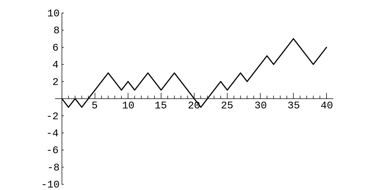
Example For our next example, we consider a problem where the exact answer is difficult to obtain but for which simulation easily gives the qualitative results. Peter and Paul play a game called heads or tails. In this game, a fair coin is tossed a sequence of times---we choose 40. Each time a head comes up Peter wins 1 penny from Paul, and each time a tail comes up Peter loses 1 penny to Paul. For example, if the results of the 40 tosses are

THTHHHHTTHTHHTTHHTTTTHHHTHHTHHHTHHHTTTHH.

Peter's winnings may be graphed as in Figure

Peter’s winnings in 40 plays of heads or tails.

Peter has won 6 pennies in this particular game. It is natural to ask for the probability that he will win [math]j[/math] pennies; here [math]j[/math] could be any even number from [math]-40[/math] to [math]40[/math]. It is reasonable to guess that the value of [math]j[/math] with the highest probability is [math]j = 0[/math], since this occurs when the number of heads equals the number of tails. Similarly, we would guess that the values of [math]j[/math] with the lowest probabilities are [math]j = \pm 40[/math].

A second interesting question about this game is the following: How many times in the 40 tosses will Peter be in the lead? Looking at the graph of his winnings (Figure), we see that Peter is in the lead when his winnings are positive, but we have to make some convention when his winnings are 0 if we want all tosses to contribute to the number of times in the lead. We adopt the convention that, when Peter's winnings are 0, he is in the lead if he was ahead at the previous toss and not if he was behind at the previous toss. With this convention, Peter is in the lead 34 times in our example. Again, our intuition might suggest that the most likely number of times to be in the lead is 1/2 of 40, or 20, and the least likely numbers are the extreme cases of 40 or 0.

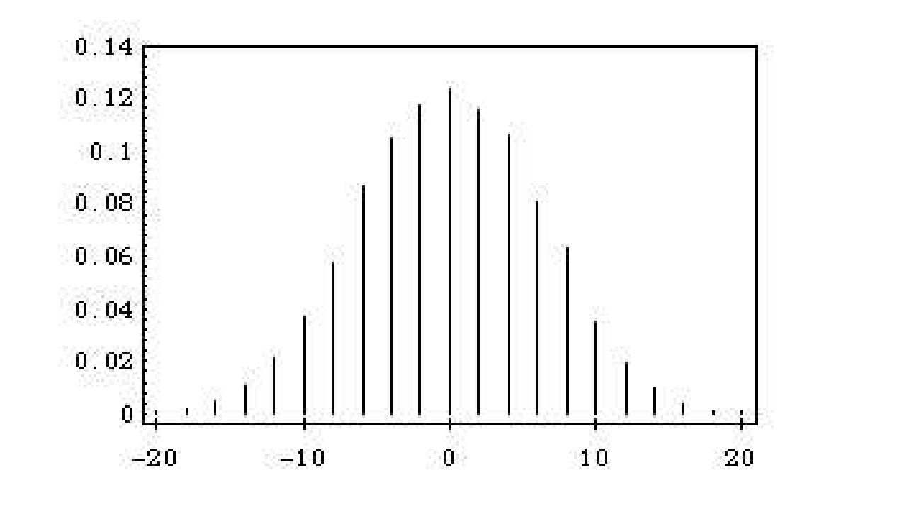
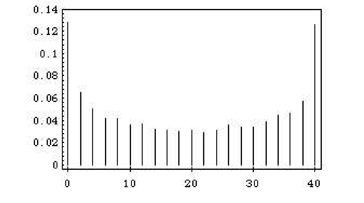
It is easy to settle this by simulating the game a large number of times and keeping track of the number of times that Peter's final winnings are [math]j[/math], and the number of times that Peter ends up being in the lead by [math]k[/math]. The proportions over all games then give estimates for the corresponding probabilities. The program HTSimulation carries out this simulation. Note that when there are an even number of tosses in the game, it is possible to be in the lead only an even number of times. We have simulated this game 10,00 times. The results are shown in Figure and Figure. These graphs, which we call spike graphs, were generated using the program Spikegraph.

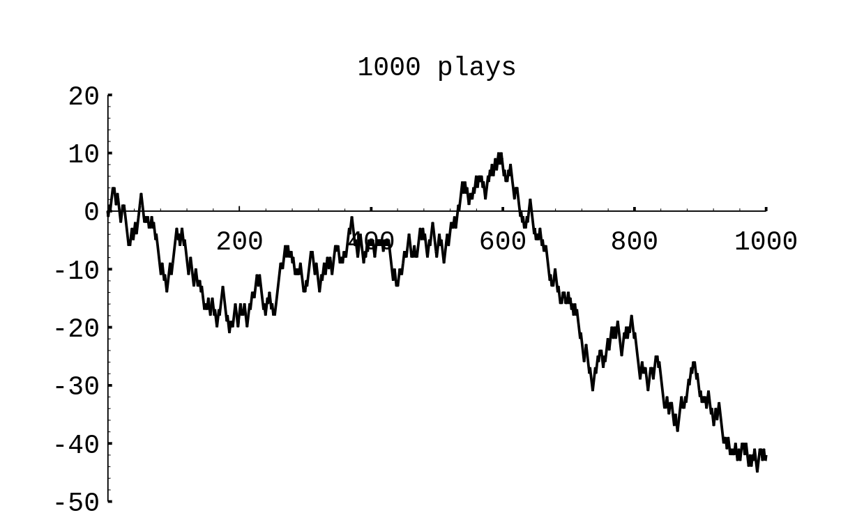
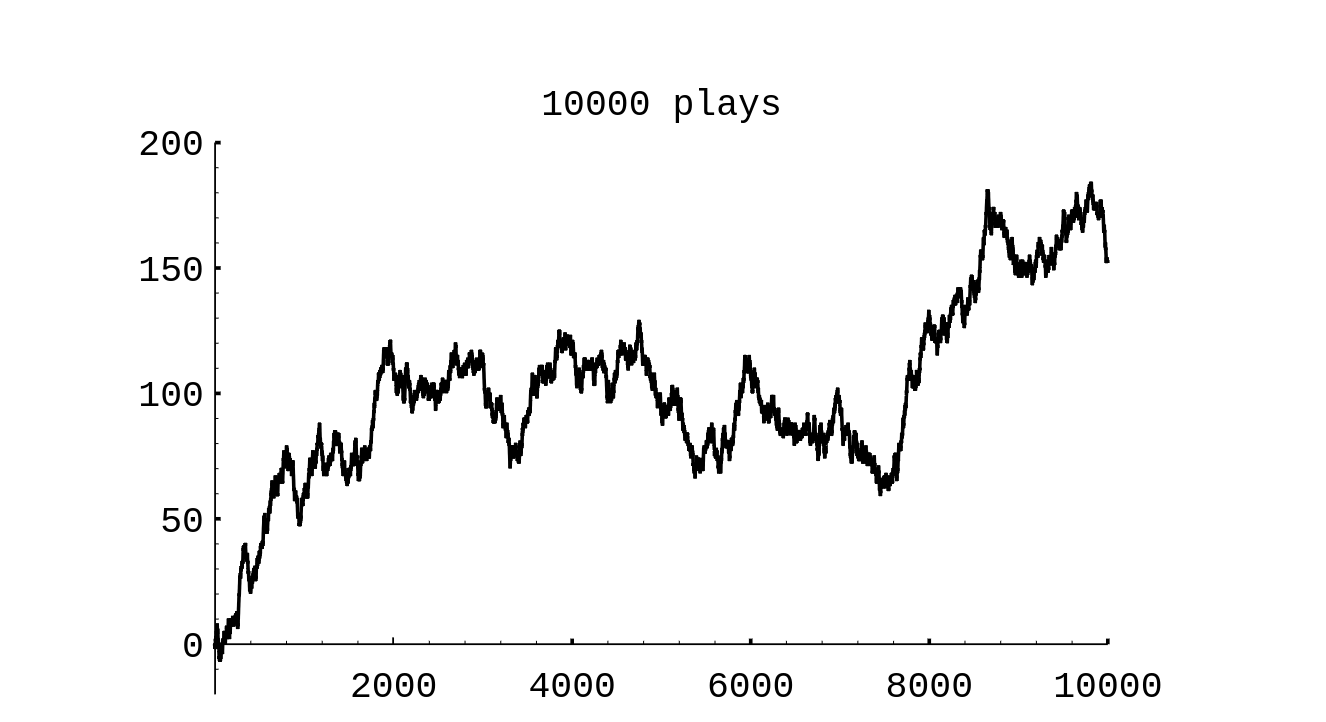
The vertical line, or spike, at position [math]x[/math] on the horizontal axis, has a height equal to the proportion of outcomes which equal [math]x[/math]. Our intuition about Peter's final winnings was quite correct, but our intuition about the number of times Peter was in the lead was completely wrong. The simulation suggests that the least likely number of times in the lead is 20 and the most likely is 0 or 40. This is indeed correct, and the explanation for it is suggested by playing the game of heads or tails with a large number of tosses and looking at a graph of Peter's winnings. In Figure we show the results of a simulation of the game, for 1000 tosses and in Figure for 10,00 tosses.

In the second example Peter was ahead most of the time. It is a remarkable fact, however, that, if play is continued long enough, Peter's winnings will continue to come back to 0, but there will be very long times between the times that this happens. These and related results will be discussed in Chapter Random walks.

In all of our examples so far, we have simulated equiprobable outcomes. We illustrate next an example where the outcomes are not equiprobable.

Distribution of winnings.

Distribution of number of times in the lead.

Peter's winnings in 1000 plays of heads or tails.

Peter's winnings in 10,000 plays of heads or tails.

Example Four horses (Acorn, Balky, Chestnut, and Dolby) have raced many times. It is estimated that Acorn wins 30 percent of the time, Balky 40 percent of the time, Chestnut 20 percent of the time, and Dolby 10 percent of the time.

We can have our computer carry out one race as follows: Choose a random number [math]x[/math]. If [math]x \lt .3[/math] then we say that Acorn won. If [math].3 \le x \lt .7[/math] then Balky wins. If [math].7 \le x \lt .9[/math] then Chestnut wins. Finally, if [math].9 \le x[/math] then Dolby wins.

The program HorseRace uses this method to simulate the outcomes of [math]n[/math] races. Running this program for [math]n = 10[/math] we found that Acorn won 40 percent of the time, Balky 20 percent of the time, Chestnut 10 percent of the time, and Dolby 30 percent of the time. A larger number of races would be necessary to have better agreement with the past experience. Therefore we ran the program to simulate 1000 races with our four horses. Although very tired after all these races, they performed in a manner quite consistent with our estimates of their abilities. Acorn won 29.8 percent of the time, Balky 39.4 percent, Chestnut 19.5 percent, and Dolby 11.3 percent of the time.

The program GeneralSimulation uses this method to simulate repetitions of an arbitrary experiment with a finite number of outcomes occurring with known probabilities.

Historical Remarks

Anyone who plays the same chance game over and over is really carrying out a simulation, and in this sense the process of simulation has been going on for centuries. As we have remarked, many of the early problems of probability might well have been suggested by gamblers' experiences.

It is natural for anyone trying to understand probability theory to try simple experiments by tossing coins, rolling dice, and so forth. The naturalist Buffon tossed a coin 4040 times, resulting in 2048 heads and 1992 tails. He also estimated the number [math]\pi[/math] by throwing needles on a ruled surface and recording how many times the needles crossed a line.

The English biologist W. F. R. Weldon recorded 26,06 throws of 12 dice, and the Swiss scientist Rudolf Wolf recorded 100,00 throws of a single die without a computer. Such experiments are very time-consuming and may not accurately represent the chance phenomena being studied. For example, for the dice experiments of Weldon and Wolf, further analysis of the recorded data showed a suspected bias in the dice. The statistician Karl Pearson analyzed a large number of outcomes at certain roulette tables and suggested that the wheels were biased. He wrote in 1894:

Clearly, since the Casino does not serve the valuable end of huge laboratory for the preparation of probability statistics, it has no scientific raison d'être. Men of science cannot have their most refined theories disregarded in this shameless manner! The French Government must be urged by the hierarchy of science to close the gaming-saloons; it would be, of course, a graceful act to hand over the remaining resources of the Casino to the Académie des Sciences for the endowment of a laboratory of orthodox probability; in particular, of the new branch of that study, the application of the theory of chance to the biological problems of evolution, which is likely to occupy so much of men's thoughts in the near future.

However, these early experiments were suggestive and led to important discoveries in probability and statistics. They led Pearson to the chi-squared test, which is of great importance in testing whether observed data fit a given probability distribution. By the early 1900s it was clear that a better way to generate random numbers was needed. In 1927, L. H. C. Tippett published a list of 41,00 digits obtained by selecting numbers haphazardly from census reports. In 1955, RAND Corporation printed a table of 1,00,00 random numbers generated from electronic noise. The advent of the high-speed computer raised the possibility of generating random numbers directly on the computer, and in the late 1940s John von Neumann suggested that this be done as follows: Suppose that you want a random sequence of four-digit numbers. Choose any four-digit number, say 6235, to start. Square this number to obtain 38,75,25. For the second number choose the middle four digits of this square (i.e., 8752). Do the same process starting with 8752 to get the third number, and so forth.

More modern methods involve the concept of modular arithmetic. If [math]a[/math] is an integer and [math]m[/math] is a positive integer, then by [math]a\ (\mbox{mod}\ m)[/math] we mean the remainder when [math]a[/math] is divided by [math]m[/math]. For example, [math]10\ ( \mbox{mod}\ 4) = 2[/math], [math]8\ (\mbox{mod}\ 2) = 0[/math], and so forth. To generate a random sequence [math]X_0,X_1, X_2,\ldots[/math] of numbers choose a starting number [math]X_0[/math] and then obtain the numbers [math]X_{n+1}[/math] from [math]X_n[/math] by the formula

[[math]] X_{n+1} = (aX_n + c)\ (\mbox{mod}\ m)\ , [[/math]]

where [math]a[/math], [math]c[/math], and [math]m[/math] are carefully chosen constants. The sequence [math] X_0, X_1,X_2, \ldots[/math] is then a sequence of integers between 0 and [math]m-1[/math]. To obtain a sequence of real numbers in [math][0,1)[/math], we divide each [math]X_j[/math] by [math]m[/math]. The resulting sequence consists of rational numbers of the form [math]j/m[/math], where [math]0 \le j \le m-1[/math]. Since [math]m[/math] is usually a very large integer, we think of the numbers in the sequence as being random real numbers in [math][0, 1)[/math].

For both von Neumann's squaring method and the modular arithmetic technique the sequence of numbers is actually completely determined by the first number. Thus, there is nothing really random about these sequences. However, they produce numbers that behave very much as theory would predict for random experiments. To obtain different sequences for different experiments the initial number [math]X_0[/math] is chosen by some other procedure that might involve, for example, the time of day.

During the Second World War, physicists at the Los Alamos Scientific Laboratory needed to know, for purposes of shielding, how far neutrons travel through various materials. This question was beyond the reach of theoretical calculations. Daniel McCracken, writing in the Scientific American, states:

The physicists had most of the necessary data: they knew the average distance a neutron of a given speed would travel in a given substance before it collided with an atomic nucleus, what the probabilities were that the neutron would bounce off instead of being absorbed by the nucleus, how much energy the neutron was likely to lose after a given collision and so on.

John von Neumann and Stanislas Ulam suggested that the problem be solved by modeling the experiment by chance devices on a computer. Their work being secret, it was necessary to give it a code name. Von Neumann chose the name “Monte Carlo.” Since that time, this method of simulation has been called the Monte Carlo Method. William Feller indicated the possibilities of using computer simulations to illustrate basic concepts in probability in his book An Introduction to Probability Theory and Its Applications. In discussing the problem about the number of times in the lead in the game of “heads or tails” Feller writes:

The results concerning fluctuations in coin tossing show that widely held beliefs about the law of large numbers are fallacious. These results are so amazing and so at variance with common intuition that even sophisticated colleagues doubted that coins actually misbehave as theory predicts. The record of a simulated experiment is therefore included.

Feller provides a plot showing the result of 10,00 plays of heads or tails similar to that in Figure. The martingale betting system described in Exercise has a long and interesting history. Russell Barnhart pointed out to the authors that its use can be traced back at least to 1754, when Casanova, writing in his memoirs, History of My Life, writes

She [Casanova's mistress] made me promise to go to the casino [the Ridotto in Venice] for money to play in partnership with her. I went there and took all the gold I found, and, determinedly doubling my stakes according to the system known as the martingale, I won three or four times a day during the rest of the Carnival. I never lost the sixth card. If I had lost it, I should have been out of funds, which amounted to two thousand zecchini.

Even if there were no zeros on the roulette wheel so the game was perfectly fair, the martingale system, or any other system for that matter, cannot make the game into a favorable game. The idea that a fair game remains fair and unfair games remain unfair under gambling systems has been exploited by mathematicians to obtain important results in the study of probability. We will introduce the general concept of a martingale in Chapter Expected Value and Variance. The word martingale itself also has an interesting history. The origin of the word is obscure. A recent version of the Oxford English Dictionary gives examples of its use in the early 1600s and says that its probable origin is the reference in Rabelais's Book One, Chapter 20:

Everything was done as planned, the only thing being that Gargantua doubted if they would be able to find, right away, breeches suitable to the old fellow's legs; he was doubtful, also, as to what cut would be most becoming to the orator---the martingale, which has a draw-bridge effect in the seat, to permit doing one's business more easily; the sailor-style, which affords more comfort for the kidneys; the Swiss, which is warmer on the belly; or the codfish-tail, which is cooler on the loins.

Dominic Lusinchi noted an earlier occurrence of the word martingale. According to the French dictionary Le Petit Robert, the word comes from the Provençal word “martegalo,” which means “from Martigues.” Martigues is a town due west of Merseille. The dictionary gives the example of “chausses à la martinguale” (which means Martigues-style breeches) and the date 1491. In modern uses martingale has several different meanings, all related to holding down, in addition to the gambling use. For example, it is a strap on a horse's harness used to hold down the horse's head, and also part of a sailing rig used to hold down the bowsprit. The Labouchere system described in Exercise is named after Henry du Pre Labouchere (1831--1912), an English journalist and member of Parliament. Labouchere attributed the system to Condorcet. Condorcet (1743--1794) was a political leader during the time of the French revolution who was interested in applying probability theory to economics and politics. For example, he calculated the probability that a jury using majority vote will give a correct decision if each juror has the same probability of deciding correctly. His writings provided a wealth of ideas on how probability might be applied to human affairs.

General references

Doyle, Peter G. (2006). "Grinstead and Snell's Introduction to Probability" (PDF). Retrieved June 6, 2024.