The Definite Integral

[math] \newcommand{\ex}[1]{\item } \newcommand{\sx}{\item} \newcommand{\x}{\sx} \newcommand{\sxlab}[1]{} \newcommand{\xlab}{\sxlab} \newcommand{\prov}[1] {\quad #1} \newcommand{\provx}[1] {\quad \mbox{#1}} \newcommand{\intext}[1]{\quad \mbox{#1} \quad} \newcommand{\R}{\mathrm{\bf R}} \newcommand{\Q}{\mathrm{\bf Q}} \newcommand{\Z}{\mathrm{\bf Z}} \newcommand{\C}{\mathrm{\bf C}} \newcommand{\dt}{\textbf} \newcommand{\goesto}{\rightarrow} \newcommand{\ddxof}[1]{\frac{d #1}{d x}} \newcommand{\ddx}{\frac{d}{dx}} \newcommand{\ddt}{\frac{d}{dt}} \newcommand{\dydx}{\ddxof y} \newcommand{\nxder}[3]{\frac{d^{#1}{#2}}{d{#3}^{#1}}} \newcommand{\deriv}[2]{\frac{d^{#1}{#2}}{dx^{#1}}} \newcommand{\dist}{\mathrm{distance}} \newcommand{\arccot}{\mathrm{arccot\:}} \newcommand{\arccsc}{\mathrm{arccsc\:}} \newcommand{\arcsec}{\mathrm{arcsec\:}} \newcommand{\arctanh}{\mathrm{arctanh\:}} \newcommand{\arcsinh}{\mathrm{arcsinh\:}} \newcommand{\arccosh}{\mathrm{arccosh\:}} \newcommand{\sech}{\mathrm{sech\:}} \newcommand{\csch}{\mathrm{csch\:}} \newcommand{\conj}[1]{\overline{#1}} \newcommand{\mathds}{\mathbb} [/math]

In defining the definite integral, we shall use the concepts of bounded sets discussed in Section 1 of Chapter 1. Recall that a number [math]u[/math] is said to be an upper bound of a set [math]S[/math] of real numbers if the inequality [math]x \leq u[/math] is satisfied for every number [math]x[/math] in [math]S[/math]. Thus the numbers 100, 5, and 1 are all upper bounds of the closed interval [math][0, 1][/math]. The Least Upper Bound Property (see page 7) states that every nonempty set of real numbers which has an upper bound has a least upper bound. For example, the number 1 is obviously the least upper bound of the interval [0,1]. Note that 1 is also the least upper bound of the open interval (0, 1). In the same way, a number [math]l[/math] is called a lower bound of [math]S[/math] provided [math]l \leq x[/math] for every [math]x[/math] in [math]S[/math]. The Greatest Lower Bound Property (see Problem 11, page 9) similarly asserts that if [math]S[/math] is nonempty and has a lower bound, then it has a greatest lower bound. Finally, a set is simply said to be bounded if it has both an upper bound and a lower bound. The notion of boundedness can be applied to functions. Specifically, a real-valued function [math]f[/math] of a real variable is said to be bounded on an interval [math]I[/math] if the following two conditions are satisfied:

• [math]I[/math] is a subset of the domain of [math]f[/math].
• There exists a real number [math]k[/math] such that [math]|f(x)| \leq k[/math], for every [math]x[/math] in [math]I[/math].

The reader should be able to supply the straightforward argument which shows that condition (ii) is equivalent to the assertion that the set [math]S[/math] of all real numbers [math]f(x)[/math] for which [math]x[/math] is in [math]I[/math] is a bounded set. To illustrate the terminology, consider the two functions [math]f[/math] and [math]g[/math] defined by [math]f(x) = x^2[/math] and [math]g(x) = \frac{1}{x}[/math]. The former is bounded on both the closed interval [0, 1] and the [math]x[/math] open interval (0, 1), whereas the latter is bounded on neither. Let [math][a, b][/math] be a closed interval, and let [math]\sigma = \{ x_0, . . ., x_n \}[/math] be a finite subset of [math][a, b][/math] which contains the endpoints [math]a[/math] and [math]b[/math]. The set [math]\sigma[/math] subdivides, or partitions, the interval into subintervals, and, for this reason, we shall call it a partition of [math][a, b][/math]. Let [math]f[/math] be a function which is bounded on the closed interval [math][a, b][/math], and let [math]\sigma =\{ x_0, . . ., x_n \}[/math] be a partition of [math][a, b][/math] in which

[[math]] a = x_0 \leq x_1 \leq ... \leq x_{n-1} \leq x_n = b. [[/math]]

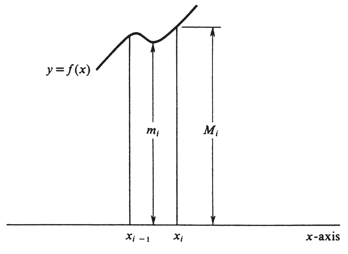
Since [math]f[/math] is bounded on the entire interval [math][a, b][/math], it is certainly bounded on each subinterval [math][x_{i - 1}, x_i][/math], for [math]i = 1, . . ., n[/math]. Hence the set [math]S[/math] consisting of all numbers [math]f(x)[/math] with [math]x[/math] in [math][x_{i-1}, x_i][/math] has a least upper bound, which we denote by [math]M_i[/math]. Similarly, of course, the set [math]S[/math] has a greatest lower bound, which we denote by [math]m_i[/math]. These numbers are illustrated for a typical subinterval in Figure. We now define two numbers [math]U_{\sigma}[/math] and [math]L_{\sigma}[/math] called, respectively, the upper sum and the lower sum of [math]f[/math] relative to the partition [math]\sigma[/math] by the formulas

[[math]] \begin{equation} \begin{array}{ll} U_\sigma &= M_{1}(x_1- x_0) + M_{2}(x_2 - x_1) + ... + M_{n}(x_{n} - x_{n-1}), \\ L_\sigma &= m_{1}(x_1- x_0) + m_{2}(x_2 - x_1) + ... + m_{n}(x_{n} - x_{n-1}). \end{array} \label{eq4.1.1} \end{equation} [[/math]]

Since [math]M_i \geq m_i[/math] and since [math](x_i - x_{i-1} \geq 0[/math], for each [math]i = 1, . . ., n[/math], it follows that

[[math]] U_{\sigma} - L_{\sigma} = (M_1 - m_1) (x_1 - x_0) + (M_2 - m_2) (x_2 - x_1) + ... + (M_n - m_n) (x_n - x_{n-1}) \geq 0. [[/math]]

Hence, we conclude that

[[math]] \begin{equation} L_{\sigma} \leq U_{\sigma}. \label{eq4.1.2} \end{equation} [[/math]]

Example

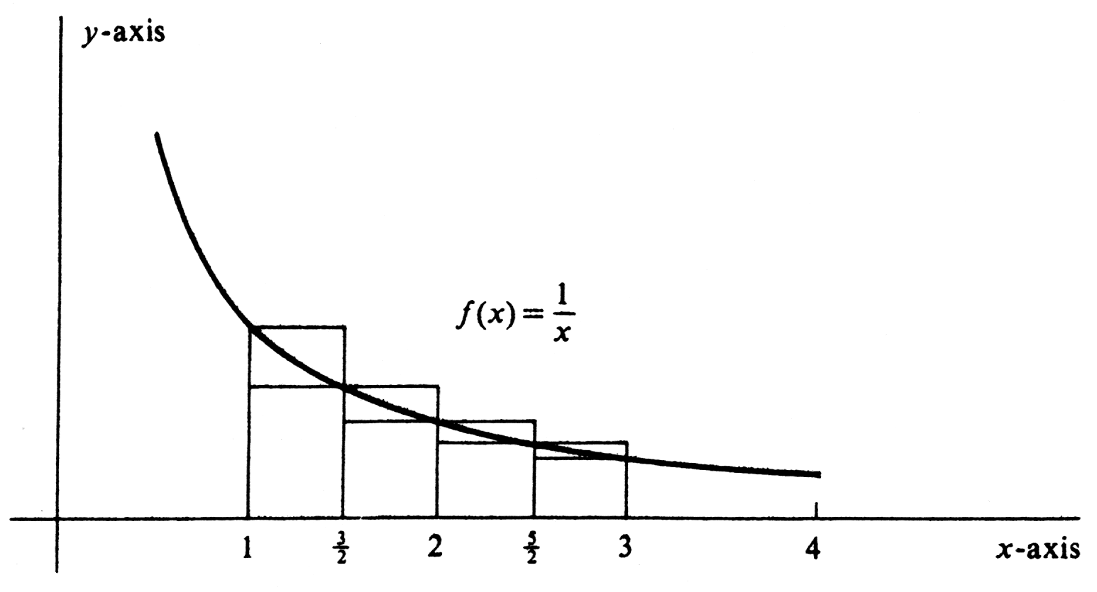
Let [math]f[/math] be the function defined by [math]f(x) = \frac{1}{x}[/math], let [math][a, b] = [1, 3][/math], and consider the partition [math]\sigma = \{ 1, \frac{2}{3}, 2, \frac{2}{5}, 3 \}[/math]. There are four subintervals, [math][1, \frac{3}{2}][/math], [math][\frac{3}{2}, 2][/math], [math][2, \frac{5}{2}][/math], and [math][\frac{5}{2}, 3][/math], and each one is of length [math]\frac{1}{2}[/math]. It is clear from Figure that the maximum value of [math]f[/math] on each subinterval occurs at the left endpoint, and the minimum value occurs at the right endpoint. Hence

[[math]] \begin{array}{l} M_1 = f(1) = 1, \;\;\; m_1 = f(\frac{3}{2}) = \frac{2}{3}, \\ \\ M_2 = f(\frac{3}{2}) = \frac{2}{3}, \;\;\; m_2 = f(2) = \frac{1}{2}, \\ \\ M_3 = f(2) = \frac{1}{2}, \;\;\; m_3 = f(\frac{5}{2}) = \frac{2}{5}, \\ \\ M_4 = f(\frac{5}{2}) = \frac{2}{5}, \;\;\; m_4 = f(3) = \frac{1}{3}. \end{array} [[/math]]

It follows that

[[math]] \begin{eqnarray*} U_{\sigma} &=& 1 \cdot \frac{1}{2} + \frac{2}{3} \cdot \frac{1}{2} + \frac{1}{2} \cdot \frac{1}{2} + \frac{2}{5} \cdot \frac{1}{2}, \\ L_{\sigma} &=& \;\;\;\;\;\;\;\;\;\;\;\; \frac{2}{3} \cdot \frac{1}{2} + \frac{1}{2} \cdot \frac{1}{2} + \frac{2}{5} \cdot \frac{1}{2} + \frac{1}{3} \cdot \frac{1}{2}. \end{eqnarray*} [[/math]]

Continuing the computation, we obtain

[[math]] \begin{eqnarray*} U_{\sigma} &=& \frac{1}{2} \Bigl(1 + \frac{2}{3} + \frac{1}{2} + \frac{2}{5} \Bigr) = \frac{1}{2} \frac{ 30 + 20 + 15 + 12}{30} = \frac{77}{60}, \\ L_{\sigma} &=& \frac{1}{2} \Bigl( \frac{2}{3} + \frac{1}{2} + \frac{2}{5} + \frac{1}{3} \Bigr) = \frac{1}{2} \frac{ 20 + 15 + 12 + 10}{30} = \frac{57}{60}, \end{eqnarray*} [[/math]]

for the values of the upper and lower sums of [math]f[/math] relative to [math]\sigma[/math].

In the paragraph preceding Example 1, it is proved that, for a given partition [math]\sigma[/math], the lower sum is less than or equal to the upper sum. We shall now prove the much stronger fact that all the lower sums are less than or equal to all the upper sums More precisely,

Theorem

Let [math]f[/math] be bounded on [math][a, b][/math]. If [math]\sigma[/math] and [math]\tau[/math] are any two partitions if [math][a, b][/math], then [math]L_{\sigma} \leq U_{\tau}[/math].

Show Proof

The argument will be divided into three parts.

(i) If [math]\tau[/math] is obtained from [math]\sigma[/math] by adjoining just one new number [math]y[/math], then [math]L_{\sigma} \leq L_{\tau} \leq U_{\tau} \leq U_{\sigma}[/math].

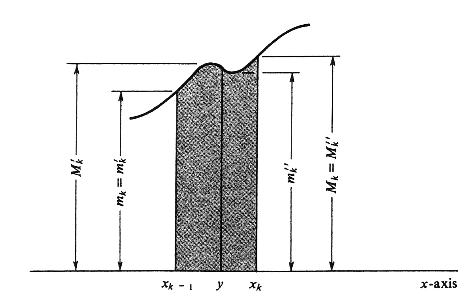
Let [math]\sigma = \{ x_0, . . . x_n \}[/math] and [math]a = x_0 \leq x_1 \leq ... \leq x_n = b[/math], and let the upper and lower sums [math]U_{\sigma}[/math] and [math]L_{\sigma}[/math] be defined as in (1), page 165. We shall assume that [math]y[/math] lies in the [math]k[/math]th subinterval [math][x_{k-1}, x_k][/math]. Then

[[math]] \tau = \{ x_0, ..., x_{k-1}, y, x_k, ..., x_n \} [[/math]]

and

[[math]] \sigma = x_0 \leq ... \leq x_{k-1} \leq y \leq x_k \leq ... \leq x_n = b. [[/math]]

Abbreviating the expressions least upper bound and greatest lower bound by l.u.b. and g.l.b., respectively, let

[[math]] \begin{eqnarray*} M_{k}' &=&\mbox{l.u.b. of the set of all numbers} \;f(x) \;\mbox{with}\; x_{k-1} \leq x \leq y,\\ M_{k}'' &=&\mbox{l.u.b. of the set of all numbers} \;f(x) \;\mbox{with}\; y \leq x \leq x_{k}, \\ m_{k}' &=&\mbox{g.l.b. of the set of all numbers} \;f(x) \;\mbox{with}\; x_{k-1} \leq x \leq y,\\ m_{k}'' &=&\mbox{g.l.b. of the set of all numbers} \;f(x) \;\mbox{with}\; y \leq x \leq x_k. \end{eqnarray*} [[/math]]

These numbers are illustrated in Figure.

The key idea in the entire proof is the fact that the least upper bound of [math]f[/math] on any set [math]S[/math] is greater than or equal to its least upper bound on any subset of [math]S[/math], and, similarly, the greatest lower bound of [math]f[/math] on [math]S[/math] is less than or equal to its greatest lower bound on a subset of [math]S[/math]. This means that

[[math]] \begin{eqnarray*} M_{k} \geq M_{k}' & \;\;\;\mbox{and}\;\;\; & M_{k} \geq M_{k}'',\\ m_{k} \leq m_{k}' & \;\;\;\mbox{and}\;\;\; & m_{k} \leq m_{k}'', \end{eqnarray*} [[/math]]

as is borne out by Figure. Hence

[[math]] \begin{eqnarray*} M_{k}(x_{k} - x_{k-1}) &=& M_{k}(x_{k} - y) + M_{k} (y - x_{k-1}) \\ &\geq& M_{k}'' (x_{k} - y) + M_{k}' (y - x_{k - 1}), \\ m_{k}(x_{k} - x_{k-1}) &=& m_{k}(x_{k} - y) + m_{k}(y - x_{k -1}) \\ &\leq& m_{k}'' (x_{k} - y) + m_{k}' (y - x_{k - 1}). \end{eqnarray*} [[/math]]

But the other terms in the upper and lower sums are the same for the two partitions. We conclude that [math]U_{\sigma} \geq U_{\tau}[/math] and that [math]L_{\sigma} \leq L_{\tau}[/math]. Since it follows from (2) that [math]L_{\tau} \leq U_{\tau}[/math], we obtain

[[math]] \begin{equation} L_{\sigma} \leq L_{\tau} \leq U_{\tau} \leq U_{\sigma}. \label{eq4.1.3} \end{equation} [[/math]]

(ii) If [math]\sigma[/math] is a subset of [math]\tau[/math], then the preceding inequalities (3) are still satisfied.

This follows by repeated applications of part (i), since the partition [math]\tau[/math] can be obtained from [math]\sigma[/math] by adjoining one number at a time.

(iii) If [math]\sigma[/math] and [math]\tau[/math] are any two partitions, then [math]L_{\sigma} \leq U_{\tau}[/math]

Both [math]\sigma[/math] and [math]\tau[/math] are subsets of the partition [math]\sigma \cup \tau[/math] consisting of their union. Hence, one application of part (ii) gives [math]L_{\sigma} \leq L_{\sigma \cup \tau}[/math], and another application yields [math]U_{\sigma \cup \tau} \leq U_{\tau}[/math]. Combining these inequalities with [math]L_{\sigma \cup \tau} \leq U_{\sigma \cup \tau}[/math], we obtain

[[math]] L_{\sigma} \leq L_{\sigma \cup \tau} \leq U_{\sigma \cup \tau} \leq U_{\tau}, [[/math]]

and the proof is complete.

■

Theorem states that, for a given function [math]f[/math] bounded on an interval [math][a, b][/math], if we consider all partitions of [math][a, b][/math], then every lower sum is less than or equal to every upper sum. It is instructive to picture the relative positions of these numbers on the real line. If we indicate each lower sum by a right hand parenthesis, “)”, and each upper sum by a left-hand parenthesis, “(”, the situation looks as shown in Figure (except that in general there are infinitely many sums of both kinds). The question naturally arises as to the existence of numbers in between the two sets, and this brings us to the definitions of integrability and of the definite integral: Let the function [math]f[/math] be bounded on the closed interval [math][a, b][/math]. Then [math]f[/math] is said to be integrable over [math][a, b][/math] if there exists one and only one number [math]J[/math] such that

[[math]] \begin{equation} L_{\sigma} \leq J \leq U_{\tau}, \label{eq4.1.4} \end{equation} [[/math]]

for any two partitions [math]\sigma[/math] and [math]\tau[/math] of [math][a, b][/math]. If [math]f[/math] is integrable over [math][a, b][/math], then the uniqbue number [math]J[/math] is called the definite integral of [math]f[/math] from [math]a[/math] to [math]b[/math], and is denoted by [math]\int_{a}^{b} f[/math]. That is,

[[math]] J = \int_{a}^{b} f. [[/math]]

Almost all the functions encountered in a first course in calculus are integrable over the closed intervals on which they are bounded. The reason is that for these functions the differences between the upper and lower sums can be made arbitrarily small by taking partitions which subdivide the interval into smaller and smaller subintervals. Many conditions which ensure that a function is integrable are known. Among these, we shall consider two [see Theorems (3.3) and (5.1)]. The second condition is continuity. We shall see that if [math]f[/math] is continuous at every point of a closed interval [math][a, b][/math], then [math]f[/math] is integrable over [math][a, b][/math]. If [math]f[/math] is a function bounded on [math][a, b][/math], there are, according to the definition, two conditions which must be satisfied for [math]f[/math] to be integrable over [math][a, b][/math]. The first is that there must exist a number [math]J[/math] such that the inequalities (4) hold for all partitions [math]\sigma[/math] and [math]\tau[/math] of the interval. The second is that there must be only one such number. It is not hard to prove that the first condition is always satisfied (see Problem 9 at the end of this section). It is the second which may fail, as the following example illustrates. Let [math]f[/math] be the function defined by

[[math]] f(x) = \left \{ \begin{array} {ll} 0 &\;\;\;\mbox{if $x$ is rational,}\\ 1 &\;\;\;\mbox{if $x$ is irrational.} \end{array} \right. [[/math]]

This function is bounded on the interval [0, 1]. However, if a is any partition whatever of [0,1], it is easy to see that [math]U_{\sigma} = 1[/math] and [math]L_{\sigma} = 0[/math]. This means that every number [math]J[/math] between, and including, 0 and 1 will satisfy (4). The function is therefore not integrable because [math]J[/math] is not unique.

Example

Assuming that the function [math]f[/math] defined by [math]f(x) = \frac{1}{x}[/math] is integrable over the interval [1, 3], prove that

[[math]] \frac{57}{60} \leq \int_{1}^{3} f \leq \frac{77}{60}. [[/math]]

This is the function and interval described in Example 1. For the partition [math]\sigma = \{ 1, \frac{3}{2}, 2, \frac{5}{2}, 3 \}[/math], we saw that [math]L_{\sigma} = \frac{57}{60}[/math] and [math]U_{\sigma} =\frac{77}{60}[/math]; hence the integral is bounded by these two numbers.

Example

Consider the function [math]f[/math] defined by [math]f(x)= x^2 [/math]. Assumingthat [math]f[/math] is integrable over the interval [0, 1], show that

[[math]] \frac{6}{25} \leq \int_{0}^{1} f \leq \frac{11}{25}. [[/math]]

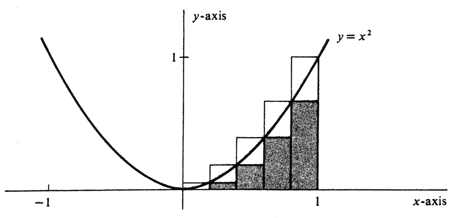
We use the partition [math]\sigma = \{ 0, \frac{1}{5},\frac{2}{5}, \frac{3}{5}, \frac{4}{5}, 1 \}[/math] and compute the upper and lower sums [math]U_{\sigma}[/math] and [math]L_{\sigma}[/math]. The points of the partition are given by [math]x_i = \frac{i}{5}[/math], for [math]i= 0, ..., 5[/math]. Hence

[[math]] x_i - x_{i-1} = \frac{1}{5}, \;\;\;\mbox{for}\;\;\; i = 1, . . ., 5. [[/math]]

Since in this case the subintervals are all of length [math]\frac{1}{5}[/math], equations (1) can be simplified to read

[[math]] \begin{eqnarray*} U_{\sigma} &=& \frac{1}{5}(M_1 + ... + M_5),\\ L_{\sigma} &=& \frac{1}{5}(m_1 + ... + m_5). \end{eqnarray*} [[/math]]

It is clear from Figure that the maximum value of [math]f[/math] on each subinterval [math][x_{i - 1}, x_i][/math] occurs at the right endpoint, and the minimum value occurs at the left endpoint. Hence [math]M_i = f(x_i)[/math] and [math]m_i = f(x_{i -1})[/math]. Since [math]f(x) = x^2[/math], we have

[[math]] \begin{array}{ll} M_{i} &= x_{i}^2 = \frac{i^2}{25} \\ m_{i} &= x_{i-1}^2 = \frac{(i - 1)^2}{25} \end{array} \left\} i = 1,..., 5. \right . [[/math]]

Thus

[[math]] \begin{eqnarray*} U_{\sigma} &=& \frac{1}{5} \Bigl( \frac{1^2}{25} + \frac{2^2}{25} + \frac{3^2}{25} + \frac{4^2}{25} + \frac{5^2}{25} \Bigr), \\ L_{\sigma} &=& \frac{1}{5} \Bigl( \frac{0^2}{25} + \frac{1^2}{25} + \frac{2^2}{25} + \frac{3^2}{25} + \frac{4^2}{25} \Bigr) . \end{eqnarray*} [[/math]]

Since [math]1^2+2^2+3^2+4^2+5^2= 55[/math] and [math]0^2+ 1^2+2^2+3^2+4^2= 30[/math], it follows that

[[math]] \begin{eqnarray*} U_{\sigma} &=& \frac{1}{5}\frac{55}{25} = \frac{11}{25},\\ L_{\sigma} &=& \frac{1}{5}\frac{30}{25} = \frac{6}{25}. \end{eqnarray*} [[/math]]

This establishes the desired bounds, since [math]L_{\sigma} \leq \int_{0}^{1} f \leq U_{\sigma}[/math].

An alternativbe notation for the integral, which we shall use interchangeably with [math]\int_{a}^{b} f[/math], is [math]\int_{a}^{b} f(x) dx[/math]. This is the traditional way of writing the integral, and its usefulness will become increasingly apparent as we go on. In a later section we shall show how the [math]dx[/math] which appears to the right of the integral sign may be interpreted as a differential. At present, however, it is important to realize that [math]dx[/math] is only a part of the notation for the integral. The variable [math]x[/math] which occurs in ia [math]\int_{a}^{b} f(x) dx[/math] is often called a dummy variable. This name serves as a reminder of the fact that the value of the integral depends only on the function [math]f[/math] and the numbers [math]a[/math] and [math]b[/math]. Its value is not determined by giving a value of [math]x[/math]. Thus

[[math]] \int_{a}^{b} f = \int_{a}^{b} f (x) dx = \int_{a}^{b} f (y) dy = \int_{a}^{b} f (t) dt = etc., [[/math]]

and [math]x[/math], [math]y[/math], and [math]t[/math] each occurs as a dummy variable. Thus the inequalities established in Examples 2 and 3 can alternatively be written

[[math]] \begin{eqnarray*} \frac{57}{60} \leq \int_{1}^{3} \frac{1}{x} dx \leq \frac{77}{60},\\ \frac{6}{25} \leq \int_{0}^{1} x^2 dx \leq \frac{11}{25}. \end{eqnarray*} [[/math]]

Although we shall not give a definition of area in this book, the basic properties of area can be used to establish its connection with the definite integral. Let the area of a set [math]P[/math] be denoted by [math]area (P)[/math]. Two basic properties are:

Theorem

The area of a set is never negative: [math]area(P) \geq 0[/math].

Theorem

If [math]P[/math] is a subset of [math]Q[/math], then [math]area(P) \leq area(Q)[/math].

In addition, we shall assume the elementary facts about the areas of rectangles.

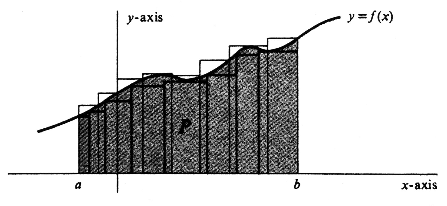
Let [math]f[/math] be a function which is integrable over the interval [math][a, b][/math], and which also satisfies the inequality [math]f(x) \geq 0[/math] for every [math]x[/math] in [math][a, b][/math]. Let [math]P[/math] be the region under the curve. That is, [math]P[/math] is the set of all points [math](x, y)[/math] in the plane such that [math]a \leq x \leq b[/math] and [math]0 \leq y \leq f(x)[/math] (see Figure). Next, consider two partitions [math]\sigma[/math] and [math]\tau[/math] of [math][a,b][/math]. The lower sum [math]L_{\sigma}[/math] is the area of the union of rectangles contained in [math]P[/math]; hence, by (1.3) we conclude that [math]L_{\sigma} \lt area (P)[/math]. Conversely, [math]P[/math] is a subset of the union of rectangles the sum of whose area is the upper sum [math]U_{\tau}[/math]. Hence [math]area (P) \leq U_{\tau}[/math], and we have shown that

[[math]] L_{\sigma} \leq area(P) \leq U_{\tau}, [[/math]]

for any two partitions [math]\sigma[/math] and [math]\tau[/math]. But the integrability of [math]f[/math] asserts that the definite integral [math]\int_{a}^{b} f(x) dx[/math] is the only number with this property. Thus we have proved

Theorem

[[math]] \int_{a}^{b} f(x) dx = area(P), \;\;\; \mbox{if}\; f(x) \geq 0\; \mbox{for every}\; x\; \mbox{in}\; [a,b]. [[/math]]

Example

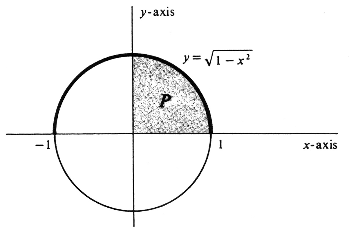
Assuming the formula for the area of a circle and the integrability of the function [math]\sqrt{1- x^2}[/math] over the interval [0, 1], compute

[[math]] \int_{0}^{1} \sqrt{1 - x^2} dx. [[/math]]

The graph of the function [math]\sqrt{1 - x^2}[/math] is the upper half of the circle [math]x^2 + y^2 = 1[/math] shown in Figure. It follows from (1.4) that the integral in question is equal [math]y[/math]-axis to one fourth of the area of the circle. Hence

[[math]] \int_{0}^{1} \sqrt{1 - x^2} dx = \frac{\pi}{4}. [[/math]]

General references

Doyle, Peter G. (2008). "Crowell and Slesnick's Calculus with Analytic Geometry" (PDF). Retrieved Oct 29, 2024.