Integrability of Monotonic Functions

[math] \newcommand{\ex}[1]{\item } \newcommand{\sx}{\item} \newcommand{\x}{\sx} \newcommand{\sxlab}[1]{} \newcommand{\xlab}{\sxlab} \newcommand{\prov}[1] {\quad #1} \newcommand{\provx}[1] {\quad \mbox{#1}} \newcommand{\intext}[1]{\quad \mbox{#1} \quad} \newcommand{\R}{\mathrm{\bf R}} \newcommand{\Q}{\mathrm{\bf Q}} \newcommand{\Z}{\mathrm{\bf Z}} \newcommand{\C}{\mathrm{\bf C}} \newcommand{\dt}{\textbf} \newcommand{\goesto}{\rightarrow} \newcommand{\ddxof}[1]{\frac{d #1}{d x}} \newcommand{\ddx}{\frac{d}{dx}} \newcommand{\ddt}{\frac{d}{dt}} \newcommand{\dydx}{\ddxof y} \newcommand{\nxder}[3]{\frac{d^{#1}{#2}}{d{#3}^{#1}}} \newcommand{\deriv}[2]{\frac{d^{#1}{#2}}{dx^{#1}}} \newcommand{\dist}{\mathrm{distance}} \newcommand{\arccot}{\mathrm{arccot\:}} \newcommand{\arccsc}{\mathrm{arccsc\:}} \newcommand{\arcsec}{\mathrm{arcsec\:}} \newcommand{\arctanh}{\mathrm{arctanh\:}} \newcommand{\arcsinh}{\mathrm{arcsinh\:}} \newcommand{\arccosh}{\mathrm{arccosh\:}} \newcommand{\sech}{\mathrm{sech\:}} \newcommand{\csch}{\mathrm{csch\:}} \newcommand{\conj}[1]{\overline{#1}} \newcommand{\mathds}{\mathbb} [/math]

Let [math]f[/math] be a given function bounded on a closed interval [math][a, b][/math]. How do we know whether or not [math]f[/math] is integrable over [math][a, b][/math], i.e., whether or not [math]\int_{a}^{b} f[/math] exists? In this section we shall give a partial answer, and also compute some integrals. Note that there is one situation where we know the answer immediately: If [math]a = b[/math], then all upper and lower sums are equal to zero. Hence [math]f[/math] is integrable, and

Theorem

[[math]] \int_{a}^{a} f = \int_{a}^{a} f (x) dx = 0. [[/math]]

So we now assume that [math]a \lt b[/math]. For every positive integer [math]n[/math], we shall denote by [math]\sigma_n[/math] the partition which subdivides [math][a, b][/math] into [math]n[/math] subintervals each of length [math]\frac{b - a}{n}[/math]. Thus [math]\sigma_n = \{x_0,... , x_n \}[/math], where

[[math]] x_i = a + \Bigl( \frac{b - a}{n} \Bigr)i, \;\;\; i = 0,..., n. [[/math]]

Moreover,

[[math]] x_i - x_{i - 1} = \frac{b - a}{n}, \;\;\; i = 1,..., n. [[/math]]

The upper and lower sums of [math]f[/math] relative to [math]\sigma_n[/math] will be denoted simply [math]U_n[/math], and [math]L_n[/math], respectively. That is, we abbreviate [math]U_{\sigma_n}[/math] by [math]U_n[/math], and in the same way [math]L_{\sigma_n}[/math] by [math]L_n[/math]. One criterion for integrability is expressed in the following theorem.

Theorem

lf [math]\lim_{n \rightarrow \infty} (U_n - L_n) = 0[/math], then [math]f[/math] is integrable over [math][a, b][/math] and

[[math]] \lim_{n \rightarrow \infty} L_n = \lim_{n \rightarrow \infty} U_n = \int_{a}^{b} f(x) dx. [[/math]]

Show Proof

We recall the basic theorem of Section 1---that the upper and lower sums of [math]f[/math] relative to any two partitions [math]\sigma[/math] and [math]\tau[/math] of the interval [math][a, b][/math] satisfy the inequality [math]L_\sigma \leq U_\tau[/math]. This implies, in particular, that any upper sum [math]U_{\tau}[/math] is an upper bound of the set L of all lower sums [math]L_{\sigma}[/math]. Hence, by the Least Upper Bound Property, the set L has a least upper bound which we denote by [math]J[/math]. Since this number [math]J[/math] is an upper bound of L, we know that [math]L_\sigma \leq J[/math] for every partition [math]\sigma[/math]. Furthermore, since [math]J[/math] is a least upper bound, we have [math]J \leq U_\tau[/math] for every partition [math]\tau[/math]. Thus

[[math]] L_\sigma \leq J \leq U_\tau, [[/math]]

for all partitions [math]\sigma[/math] and [math]\tau[/math] of [math][a, b][/math]. As a special case of these inequalities, we have

[[math]] \begin{equation} L_{n} \leq J \leq U_{n}, \;\;\; \mbox{for every positive integer}\; n. \label{eq4.3.1} \end{equation} [[/math]]

Since by hypothesis [math]\lim_{n \rightarrow \infty} (U_n - L_n) = 0[/math], it follows that this number [math]J[/math] is the only number which can lie between all upper and lower sums. Hence, by the definition, [math]f[/math] is integrable over [math][a, b][/math] and [math]J = \int_{a}^{b} f(x) dx[/math]. From (1) we obtain the inequalities

[[math]] 0 \leq J - L_n \leq U_n - L_n, \;\;\;\mbox{for every positive integer}\; n. [[/math]]

Since the right side of the above inequalities approaches zero, the expression in the middle is caught in a squeeze and must also approach zero. Hence [math]\lim_{n \rightarrow \infty} (J - L_n) = 0[/math], or, equivalently,

[[math]] \lim_{n \rightarrow \infty} L_n = J = \int_{a}^{b} f(x) dx. [[/math]]

Finally, consider the identity [math]U_n = J + (U_n - L_n) - (J - L_n)[/math]. Since the two expressions in parentheses approach zero, it follows that

[[math]] \lim_{n \rightarrow \infty} U_n = J = \int_{a}^{b} f(x)dx, [[/math]]

and the proof is complete.

■

An important class of functions to which the preceding theorem can be readily applied, and which we now define, is the class of monotonic functions. To begin with, a real-valued function [math]f[/math] is said to be increasing on an interval [math]I[/math] if the domain of [math]f[/math] contains [math]I[/math] as a subset and if, for every [math]x_1[/math] and [math]x_2[/math] in [math]I[/math],

[[math]] \begin{equation} x_1 \leq x_2 \;\;\;\mbox{implies}\;\;\; f(x_1) \leq f(x_2). \label{eq4.3.2} \end{equation} [[/math]]

If (2) holds for every [math]x_1[/math] and [math]x_2[/math] in the entire domain of [math]f[/math], we say simply that [math]f[/math] is an increasing function. Companion definitions are obtained by simultaneously replacing the second inequality in (2) by [math]f(x_1) \geq f(x_2)[/math] and the word increasing by the word decreasing. For example, the function [math]f[/math] defined by [math]f(x) = x^2[/math] is increasing on the interval [math][0, \infty)[/math] and decreasing on the interval [math](-\infty, 0][/math]. The function g defined by [math]g(x) = - 2x + 1[/math] is a decreasing function. Note that, according to our definition, a constant function is both increasing and decreasing. Thus “increasing,” as it is used here, literally means “nondecreasing,” and in the same way “decreasing” means “nonincreasing.” A monotonic function is one which is either increasing or decreasing. Similarly, a function is monotonic on an interval if it is either increasing or decreasing on the interval. For such functions it is not difficult to prove the following integrability theorem.

Theorem

If the function [math]f[/math] is monotonic on the closed interval [math][a, b][/math], then [math]f[/math] is integrable over [math][a, b][/math]. Specifically, [math]\lim_{n \rightarrow \infty} (U_n - L_n) = 0[/math].

Show Proof

{{{4}}}

■

Example

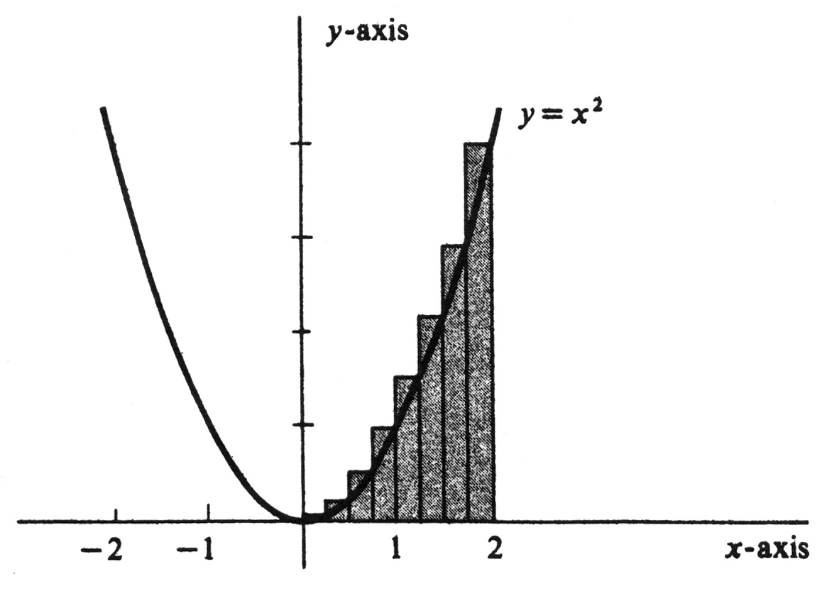
Evaluate [math]\int_{0}^{2} x^2 dx[/math]. The function [math]f[/math] to be integrated is defined by [math]f(x) = x^2[/math], and the interval of integration is [0, 2]. Since [math]f[/math] is increasing on the interval, the integral certainly exists. The partition [math]\sigma_n = \{x_0, ..., x_n \}[/math] which subdivides [0, 2] into [math]n[/math] subintervals of equal length is given by

[[math]] x_i = a+ \frac{b -a}{n} i=0+\frac{2}{n} i = \frac{2i}{n}, [[/math]]

for each [math]i = 0, . . ., n[/math]. Moreover,

[[math]] x_{i} - x_{i - 1} = \frac{b-a}{n} = \frac{2}{n}, \;\;\; i = 1, . . ., n. [[/math]]

It follows from Theorems (3.2) and (3.3) that

[[math]] \int_{0}^2 x^2 dx = \lim_{n \rightarrow \infty} U_n = \lim_{n \rightarrow \infty} L_n. [[/math]]

That is, we may compute the integral using either the lower or the upper sums. Choosing the latter, we observe from Figure that, on each subinterval [math][x_{i - 1}, x_i][/math], the function [math]f[/math] has its maximum value at the right endpoint, i.e., at [math]x_i[/math]. Hence

[[math]] M_i = f(x_i),\;\;\; i= 1,...,n. [[/math]]

Since [math]f(x_i) = x_{i}^2[/math] and since [math]x_i = \frac{2i}{n}[/math], it follows that [math]M_i = x_{i}^2 = \frac{4i^2}{n^2}[/math]. Substituting in the formula for the upper sum,

[[math]] U_n = \sum_{i=1}^{n} M_i (x_i - x_{i - 1}), [[/math]]

we obtain

[[math]] U_n = \sum_{i=1}^{n} \Bigl( \frac{4i^2}{n^2} \Bigr) \Bigl( \frac{2}{n} \Bigr) = \sum_{i=1}^{n} \frac{8i^2}{n^3} = \frac{8}{n^3} \sum_{i=1}^{n} i^2. [[/math]]

From (2.5), we have

[[math]] \sum_{i=1}^{n} i^2 = \frac{n(n + 1)(2n + 1)}{6} = \frac{ 2n^3 + 3n^2 + n}{6}. [[/math]]

Hence

[[math]] U_n = \frac{8}{n^3} \frac{2n^3 + 3n^2 + n}{6} = \frac{4}{3} \Bigl( 2 + \frac{3}{n} + \frac{1}{n^2} \Bigr), [[/math]]

and so

[[math]] \lim_{n \rightarrow \infty} U_n = \lim_{n \rightarrow \infty} \frac{4}{3} \Bigl( 2 + \frac{3}{n} + \frac{1}{n^2} \Bigr) = \frac{4}{3} \cdot 2 = \frac {8}{3}. [[/math]]

We conclude that

[[math]] \int_{0}^{2} x^2 dx = \frac{8}{3}. [[/math]]

File:Guide c5467 scanfig4 10.png

It was shown in Section 1 that the integral of a nonnegative function is equal to the area under its graph. It follows from the above example that the area of the region bounded by the parabola [math]y = x^2[/math], the [math]x[/math]-axis, and the line [math]x = 2[/math] is equal to [math]\frac{8}{3}[/math]. Example

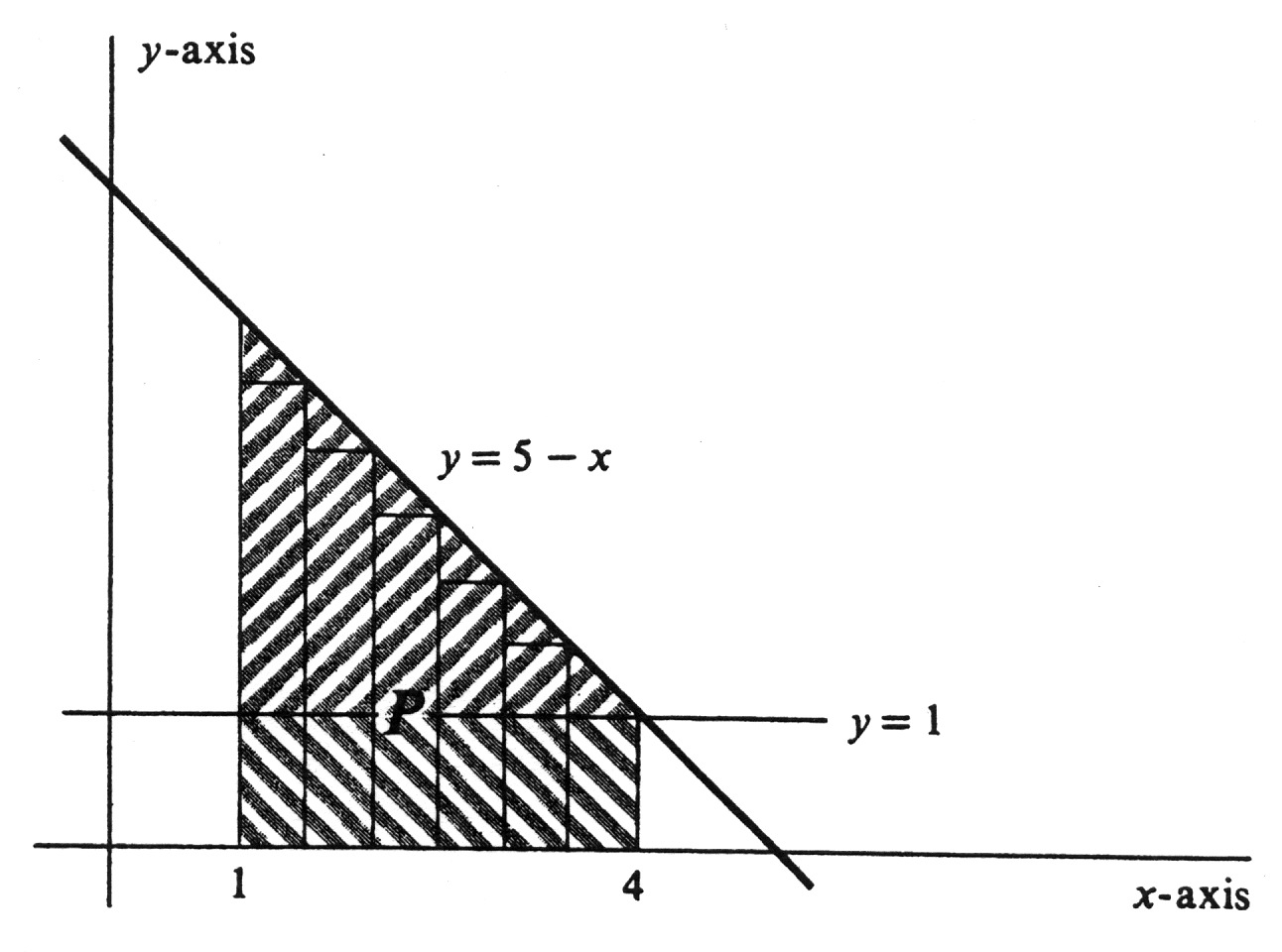
Evaluate [math]\int_{1}^{4} (5 - x) dx[/math]. The function [math]f[/math], defined by [math]f(x) = 5 - x[/math], is linear and decreasing on the interval [1, 4]. Its graph is shown in Figure. The partition [math]\sigma_{n} = \{ x_{0}, . . ., x_{n} \}[/math] subdivides the interval [1, 4] into subintervals of length [math]\frac{4 - 1}{n} = \frac{3}{n}[/math], and the points are given by

[[math]] x_{i} = 1 + \Bigl(\frac{3}{n}\Bigr) i, \;\;\; i = 0, . . . , n. [[/math]]

In addition,

[[math]] x_{i} - x_{i-1} = \frac{3}{n}, \;\;\; i = 1, ... , n. [[/math]]

We shall compute the integral as a limit of lower sums, and it follows from Theorems (3.2) and (3.3) that

[[math]] \int_{1}^{4} (5 - x)dx = \lim_{n \rightarrow \infty} L_n. [[/math]]

File:Guide c5467 scanfig4 11.png

Since [math]f[/math] is decreasing, its minimum value on each subinterval [math][x_{i-1}, x_i][/math] occurs at the right endpoint. Hence

[[math]] m_i = f(x_i), \;\;\; i= 1,...,n. [[/math]]

We have [math]x_i = 1 +\frac{3i}{n}[/math] and [math]f(x_i) = 5 - x_i[/math], and so

[[math]] m_i= 5 - \Bigl( 1 + \frac{3i}{n} \Bigr) = 4 - \frac{3i}{n}. [[/math]]

Since [math]x_{i} - x_{i-1} = \frac{3}{n}[/math], we get

[[math]] L_n = \sum_{i=1}^{n} m_{i}(x_{i} - x_{i-1}) = \sum_{i=1}^{n} \Bigl( 4 - \frac{3i}{n} \Bigr) \frac{3}{n}. [[/math]]

The rest of the problem uses the manipulative techniques of the summation convention.

[[math]] \begin{eqnarray*} L_n &=& \sum_{i=1}^{n} \Bigl( 4 - \frac{3i}{n} \Bigr) \frac{3}{n} = \sum_{i=1}^{n} \Bigl( \frac{12}{n} - \frac{9i}{n^2} \Bigr)\\ &=& \sum_{i=1}^{n} \frac{12}{n} - \sum_{i=1}^{n} \frac{9i}{n^2} \\ &=& \frac{12}{n} \sum_{i=1}^{n} 1 - \frac{9}{n^2} \sum_{i=1}^{n} i. \end{eqnarray*} [[/math]]

since [math]\sum_{i=1}^{n} 1 = n[/math] and since [math]\sum_{i=1}^{n} i = \frac{n(n + 1)}{2}[/math], we get

[[math]] \begin{eqnarray*} L_n &=& \frac{12}{n} - \frac{9}{n^2} \frac{ n(n+ 1)}{2} \\ &=&12 - \frac{9}{2} \Bigl(1 + \frac{1}{n} \Bigr) . \end{eqnarray*} [[/math]]

But it is easy to see that

[[math]] \lim_{n \rightarrow \infty} \Bigl [12 - \frac{9}{2} \Bigl( 1 + \frac{1}{n} \Bigr) \Bigr] = 12 - \frac{9}{2} = 7 \frac{1}{2}, [[/math]]

and we finally conclude that

[[math]] \int_{1}^{4} (5 - x) dx = \lim_{n \rightarrow \infty} L_n = 7 \frac{1}{2}. [[/math]]

This answer can be checked by looking at Figure. The value of the integral is equal to the area of the shaded region [math]P[/math], which is divided by the horizontal line [math]y = 1[/math] into two pieces: a right triangle sitting on top of a rectangle. The area of the triangle is [math]\frac{1}{2} (3 \cdot 3) = \frac{9}{2}[/math], and that of the rectangle is [math]3 \cdot 1 = 3[/math]. Hence

[[math]] \int_{1}^{4} (5 - x) dx = area(P) = \frac{9}{2} + 3 = 7\frac{1}{2}. [[/math]]

The excessive lengths of the computations in Examples 1 and 2 make it obvious that some powerful techniques are needed to streamline the process of evaluating definite integrals. The advent of modern high-speed computers is one answer to the problem, and occasionally, as in Example 2, a simple formula for area will do the trick. The classical solution to the problem, however, is the Fundamental Theorem of Calculus, which we shall study in detail in Section 5.

General references

Doyle, Peter G. (2008). "Crowell and Slesnick's Calculus with Analytic Geometry" (PDF). Retrieved Oct 29, 2024.