Average Value of a Function

[math] \newcommand{\ex}[1]{\item } \newcommand{\sx}{\item} \newcommand{\x}{\sx} \newcommand{\sxlab}[1]{} \newcommand{\xlab}{\sxlab} \newcommand{\prov}[1] {\quad #1} \newcommand{\provx}[1] {\quad \mbox{#1}} \newcommand{\intext}[1]{\quad \mbox{#1} \quad} \newcommand{\R}{\mathrm{\bf R}} \newcommand{\Q}{\mathrm{\bf Q}} \newcommand{\Z}{\mathrm{\bf Z}} \newcommand{\C}{\mathrm{\bf C}} \newcommand{\dt}{\textbf} \newcommand{\goesto}{\rightarrow} \newcommand{\ddxof}[1]{\frac{d #1}{d x}} \newcommand{\ddx}{\frac{d}{dx}} \newcommand{\ddt}{\frac{d}{dt}} \newcommand{\dydx}{\ddxof y} \newcommand{\nxder}[3]{\frac{d^{#1}{#2}}{d{#3}^{#1}}} \newcommand{\deriv}[2]{\frac{d^{#1}{#2}}{dx^{#1}}} \newcommand{\dist}{\mathrm{distance}} \newcommand{\arccot}{\mathrm{arccot\:}} \newcommand{\arccsc}{\mathrm{arccsc\:}} \newcommand{\arcsec}{\mathrm{arcsec\:}} \newcommand{\arctanh}{\mathrm{arctanh\:}} \newcommand{\arcsinh}{\mathrm{arcsinh\:}} \newcommand{\arccosh}{\mathrm{arccosh\:}} \newcommand{\sech}{\mathrm{sech\:}} \newcommand{\csch}{\mathrm{csch\:}} \newcommand{\conj}[1]{\overline{#1}} \newcommand{\mathds}{\mathbb} [/math]

Let [math]f[/math] be a real-valued function of a real variable which is bounded on the closed interval [math][a, b][/math]. Furthermore, let [math]f[/math] be integrable over [math][a, b][/math]. Then the mean, or average value, of [math]f[/math] on the interval [math][a, b][/math] will be denoted by [math]M_a^b(f)[/math] and is defined by

[[math]] M_a^b(f) = \left\{ \begin{array}{ll} \frac{1}{b - a} \int_a^b f, &\;\;\; \mbox{if}\; a \lt b,\\ f(a), &\;\;\; \mbox{if}\; a = b. \end{array} \right . [[/math]]

If [math]a \lt b[/math], then it follows at once from the definition that

[[math]] (b - a)M_a^b(f) = \int_a^b f . [[/math]]

This equation is also true if [math]a = b[/math], for then,both sides are equal to zero. We conclude that

Theorem

[[math]] \int_a^b f = (b - a)M_a^b(f). [[/math]]

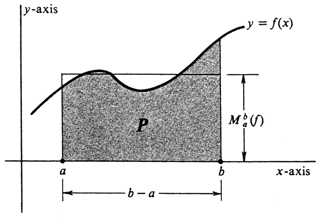
If [math]f[/math] is nonnegative on [math][a, b][/math], i.e., if [math]f(x) \geq 0[/math] for every [math]x[/math] such that [math]a \leq x \leq b[/math], then (1.1) yields a good geometric interpretation of the mean [math]M_a^b(f)[/math]. Let [math]P[/math] be the set of all points [math](x,y)[/math] such that [math]a \leq x \leq b[/math] and [math]0 \leq y \leq f(x)[/math], as shown in Figure 1. Then

[[math]] area(P) = \int_a^b f = (b - a)M_a^b(f). [[/math]]

It follows that [math]M_a^b(f)[/math] is equal to the height of a rectangle with the same base and the same area as [math]P[/math].

File:Guide c5467 scanfig8 1.png

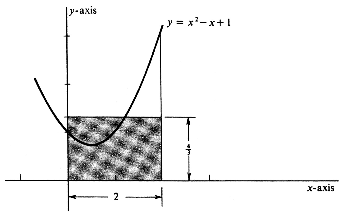
Example Let [math]f[/math] be the function defined by [math]f(x) = x^2 - x + 1[/math]. Find the average value of [math]f[/math] on the interval [math][0, 2][/math], draw the graph of [math]f[/math], and show on it the rectangle with base [math][0, 2][/math] and area equal to the area under the curve. The graph is shown in Figure 2. The mean, or average value, of [math]f[/math] is given by

[[math]] \begin{eqnarray*} M_0^2( f ) &=& \frac{1}{2 - 0} \int_0^2 f (x) dx\\ &=& \frac{1}{2} \int_0^2 (x^2 - x + 1)dx \\ &=& \frac{1}{2}(\frac{x^3}{3} - \frac{x^2}{2} + x) \big|_0^2 = \frac{4}{3} . \end{eqnarray*} [[/math]]

File:Guide c5467 scanfig8 2.png

The words “mean” and “average value” are common in our vocabularies and have intuitive meaning for most of us. To use them as names for [math]M_a^b(f)[/math] is a sensible thing to do only if this quantity, as we have defined it, has the properties we associate with these words. We shall now show that it does. First, let us verify that the average value of a velocity function agrees with our earlier definition of average velocity. We consider a particle moving along a straight line, which we take to be a coordinate axis. The position and instantaneous velocity of the particle at time [math]t[/math] are denoted by [math]s(t)[/math] and [math]v(t)[/math], respectively, and we know that [math]s'(t) = v(t)[/math]. Suppose that the interval of motion is from time [math]t = a[/math] to time [math]t = b[/math] and that [math]a \lt b[/math]. Assuming that [math]v[/math] is a continuous function, we have

[[math]] \int_a^b v(t) dt = s(b) - s(a). [[/math]]

According to the definition on page 104, the average velocity [math]v_{av}[/math] is equal to

[[math]] v_{av} = \frac{s(b) - s(a)}{b - a} . [[/math]]

The mean, or average value, of the function [math]v[/math] on the interval [math][a, b][/math] is given by

[[math]] \begin{eqnarray*} M_a^b(v) &=& \frac{1}{b-a} \int_a^b v(t) dt\\ &=& \frac{s(b) - s(a)}{b-a} = v_{av}. \end{eqnarray*} [[/math]]

Hence the two definitions agree. The basic properties of the average value of a function correspond closely to the basic properties of the definite integral as they are enumerated at the beginning of Section 4 of Chapter 4. To begin with, we would expect a function which is constant on an interval to have, on that interval, an average value equal to the constant value of the function. The following proposition states that this is so.

Theorem

If [math]f(x) = k[/math] for every [math]x[/math] in the interval [math][a, b][/math], then [math]M_a^b (f) = k[/math].

The proof is an immediate corollary of the definition of the mean [math]M_a^b (f)[/math] and of Theorem (4.1), page 191. The reader should supply the details. If one function is less than or equal to another function on some interval, then the lesser one should have the smaller average value. Thus we expect the theorem:

Theorem

If [math]f[/math] and [math]g[/math] are integrable over [math][a, b][/math] and if [math]f (x) \leq g(x)[/math] for every [math]x[/math] in [math][a, b][/math], then [math]M_a^b (f) \leq M_a^b (g)[/math].

The proof follows easily from Theorem (4.3), page 191. We introduce the third property of the average value of a function by means of an example. Suppose that on a 5-hour automobile trip the average velocity is 45 miles per hour during the first 3 hours and 30 during the last 2 hours. What is the average velocity for the whole trip? To get the answer, we observe that the total distance traveled is

[[math]] 45 \cdot 3 + 30 \cdot 2 = 195 \;\mbox{miles.} [[/math]]

The average velocity over 5 hours is, therefore,

[[math]] \frac{195}{5} = 39 \;\mbox{mph.} [[/math]]

If we denote the instantaneous velocity of the automobile by [math]v(t)[/math], and assume that the trip began at time [math]t = 0[/math], then we can express the fact that the average velocity over the first 3 hours was 45 miles per hour by the equation [math]M_0^3(v) = 45[/math]. Similarly, we are given [math]M_3^5(v) = 30[/math] and have shown that [math]M_0^5(v) = 39[/math]. Since [math]3 \cdot 45 + 2 \cdot 30 = 5 \cdot 39[/math], we can write

[[math]] (3 - 0)M_0^3(v) + (5 - 3)M_3^5(v) = (5 - 0)M_0^5(v). [[/math]]

Abstracting from this example, we conclude that the average value of a function should have the property expressed in the proposition:

Theorem

If [math]f[/math] is integrable over [math][a, b][/math] and [math][b, c][/math], then

[[math]] (b - a)M_a^{b}(f) + (c - b)M_b^{c}(f) = (c - a)M_a^{c}(f). [[/math]]

Show Proof

Since [math](b - a)M_a^b(f) = \int_a^b f[/math], the conclusion of (1.4) is equivalent to the equation

[[math]] \int_a^b f + \int_b^c f = \int_a^c f . [[/math]]

But this is one of the basic properties of the definite integral [see Theorem (4.2), page 191], so the proof is complete.

■

The next theorem states the properties of the mean corresponding to Theorems (4.4) and (4.5), page 191.

Theorem

If [math]f[/math] and [math]g[/math] are integrable over [math][a, b][/math] and if [math]k[/math] is any real number, then

1. [math]M_a^b(kf)= kM_a^b(f),[/math]
2. [math]M_a^b(f + g) = M_a^b(f ) + M_a^b(g).[/math]

The proofs are left as exercises.

Example

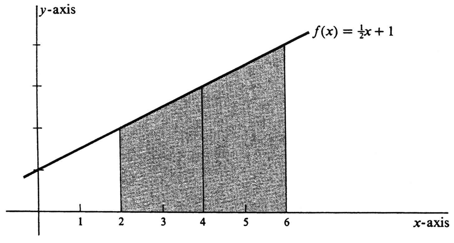
Let us see whether the definition of average value of a function agrees with our intuition in a simple example. Let [math]f[/math] be the linear function defined by

[[math]] f(x) = \frac{1}{2} x + 1, [[/math]]

whose graph is shown in Figure 3. What is the average value of [math]f[/math] between 2 and 6?

File:Guide c5467 scanfig8 3.png

We have [math]f(2) = \frac{1}{2} \cdot 2 + 1 = 2[/math] and [math]f(6) = \frac{1}{2} \cdot 6 + 1 = 4[/math]. Since the graph of [math]f[/math] is a straight line, the region below the curve is a trapezoid. It would seem natural for the average value of [math]f[/math] on the interval to be the length of the median, which is given by

[[math]] \frac{f(2) + f(6)}{2} = \frac{2 + 4}{2} = 3. [[/math]]

Computation of [math]M_2^6(f)[/math] yields

[[math]] \begin{eqnarray*} M_2^6(f) &=& \frac{1}{6 - 2} \int_2^6 (\frac{1}{2}x + 1)dx \\ &=& \frac{1}{4} (\frac{x^2}{4} + x)\Big|_2^6 \\ &=& \frac{1}{4} [( \frac{36}{4} + 6) - (\frac{4}{4} + 2)] \\ &=& \frac{1}{4} (15 - 3) = 3. \end{eqnarray*} [[/math]]

In motivating the definition of the mean, or average value, of a function, we have seen its very close connection with the definite integral. Since a beginning student of calculus probably has a greater feeling for the idea of average than for that of an integral, it is fruitful to reverse our point of view. That is, if we were to ask the question “What really is the definite integral of a function?”, one answer is that it is a weighted average. Specifically, as stated in (1.1), the integral [math]\int_a^bf[/math] is equal to the product of [math]b - a[/math] and the average value of [math]f[/math] on the interval [math][a, b][/math]. We conclude this section with a theorem which is sometimes called the integral form of the Mean Value Theorem. It asserts that if [math]f[/math] is continuous, the number [math]M_a^b(f)[/math], which we have called an average value, is quite literally the value of the function [math]f[/math] for some number between [math]a[/math] and [math]b[/math].

INTEGRAL FORM OF MEAN VALUE THEOREM

If [math]a \lt b[/math] and if [math]f[/math] is continuous on the interval [math][a, b][/math], then there exists a number [math]c[/math] such that [math]a \lt c \lt b[/math] and [math]M_a^b(f) = f(c)[/math].

Show Proof

Since [math]f[/math] is continuous at every point of [math][a, b][/math], it follows by the Fundamental Theorem of Calculus that the function [math]F[/math], defined by

[[math]] F(x) = \int_a^b f(t) dt, \;\;\;\mbox{for every $x$ in $[a, b]$,} [[/math]]

is differentiable. Furthermore,

[[math]] F'(x) = f (x), \;\;\;\mbox{for every $x$ in $[a, b]$.} [[/math]]

A differentiable function is necessarily continuous [see (6.1), page 55], and so [math]F[/math] more than satisfies the hypotheses of the Mean Value Theorem, (5.2), page 113. That theorem therefore implies that there exists a number [math]c[/math] such that [math]a \lt c \lt b[/math] and

[[math]] F(b) - F(a) = (b - a)F'(c). [[/math]]

But [math]F'(c) = f(c)[/math], and

[[math]] F(b) - F(a) = \int_a^b f(x)dx. [[/math]]

Hence

[[math]] \int_a^b f (x) dx = (b - a) f(c), [[/math]]

and so

[[math]] f(c) = \frac{1}{b - a} \int_a^b f(x) dx = M_a^b(f). [[/math]]

This completes the proof.

■

General references

Doyle, Peter G. (2008). "Crowell and Slesnick's Calculus with Analytic Geometry" (PDF). Retrieved Oct 29, 2024.