Bagging, Boosting, and Random Forests
Bootstrap aggregating, also called bagging (from bootstrap aggregating), is a machine learning ensemble meta-algorithm designed to improve the stability and accuracy of machine learning algorithms used in statistical classification and regression. It also reduces variance and helps to avoid overfitting. Although it is usually applied to decision tree methods, it can be used with any type of method. Bagging is a special case of the model averaging approach.
Description of the technique
Given a standard training set [math]D[/math] of size [math]n[/math], bagging generates [math]m[/math] new training sets [math]D_i[/math], each of size [math]n[/math], by sampling from [math]D[/math] uniformly and with replacement. By sampling with replacement, some observations may be repeated in each [math]D_i[/math]. If [math]n=n'[/math], then for large [math]n[/math] the set [math]D_i[/math] is expected to have the fraction (1 - 1/e) (≈63.2%) of the unique examples of [math]D[/math], the rest being duplicates.[1] This kind of sample is known as a bootstrap sample. Sampling with replacement ensures each bootstrap is independent from its peers, as it does not depend on previous chosen samples when sampling. Then, [math]m[/math] models are fitted using the above [math]m[/math] bootstrap samples and combined by averaging the output (for regression) or voting (for classification).
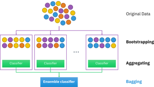
Bagging leads to "improvements for unstable procedures",[2] which include, for example, artificial neural networks, classification and regression trees, and subset selection in linear regression.[3] Bagging was shown to improve preimage learning.[4][5] On the other hand, it can mildly degrade the performance of stable methods such as K-nearest neighbors.[2]
Creating the bootstrap dataset
The bootstrap dataset is made by randomly picking objects from the original dataset. Also, it must be the same size as the original dataset. However, the difference is that the bootstrap dataset can have duplicate objects. Here is simple example to demonstrate how it works along with the illustration below:
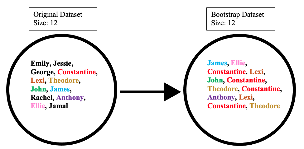
Suppose the original dataset is a group of 12 people. These guys are Emily, Jessie, George, Constantine, Lexi, Theodore, John, James, Rachel, Anthony, Ellie, and Jamal.
By randomly picking a group of names, let us say our bootstrap dataset had James, Ellie, Constantine, Lexi, John, Constantine, Theodore, Constantine, Anthony, Lexi, Constantine, and Theodore. In this case, the bootstrap sample contained four duplicates for Constantine, and two duplicates for Lexi, and Theodore.
Creating the out-of-bag dataset
The out-of-bag dataset represents the remaining people who were not in the bootstrap dataset. It can be calculated by taking the difference between the original and the bootstrap datasets. In this case, the remaining samples who were not selected are Emily, Jessie, George, Rachel, and Jamal. Keep in mind that since both datasets are sets, when taking the difference the duplicate names are ignored in the bootstrap dataset. The illustration below shows how the math is done:

Example: ozone data
To illustrate the basic principles of bagging, below is an analysis on the relationship between ozone and temperature (data from Rousseeuw and Leroy (1986), analysis done in R).
The relationship between temperature and ozone appears to be nonlinear in this data set, based on the scatter plot. To mathematically describe this relationship, LOESS smoothers (with bandwidth 0.5) are used. Rather than building a single smoother for the complete data set, 100 bootstrap samples were drawn. Each sample is composed of a random subset of the original data and maintains a semblance of the master set’s distribution and variability. For each bootstrap sample, a LOESS smoother was fit. Predictions from these 100 smoothers were then made across the range of the data. The black lines represent these initial predictions. The lines lack agreement in their predictions and tend to overfit their data points: evident by the wobbly flow of the lines.
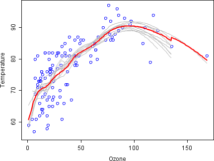
By taking the average of 100 smoothers, each corresponding to a subset of the original data set, we arrive at one bagged predictor (red line). The red line's flow is stable and does not overly conform to any data point(s).
Random Forests
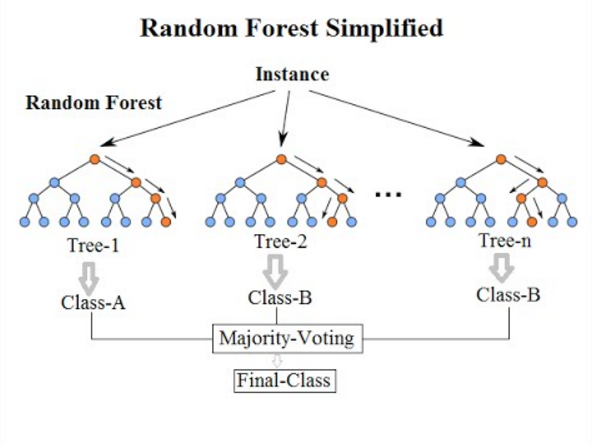
Random forests or random decision forests is an ensemble learning method for classification, regression and other tasks that operates by constructing a multitude of decision trees at training time. For classification tasks, the output of the random forest is the class selected by most trees. For regression tasks, the mean or average prediction of the individual trees is returned.[6][7] Random decision forests correct for decision trees' habit of overfitting to their training set.Template:R:587–588 Random forests generally outperform decision trees, but their accuracy is lower than gradient boosted trees. However, data characteristics can affect their performance.[8][9]
The first algorithm for random decision forests was created in 1995 by Tin Kam Ho[6] using the random subspace method,[7] which, in Ho's formulation, is a way to implement the "stochastic discrimination" approach to classification proposed by Eugene Kleinberg.[10][11][12]
An extension of the algorithm was developed by Leo Breiman[13] and Adele Cutler,[14] who registered[15] "Random Forests" as a trademark in 2006 (Template:As of, owned by Minitab, Inc.).[16] The extension combines Breiman's "bagging" idea and random selection of features, introduced first by Ho[6] and later independently by Amit and Geman[17] in order to construct a collection of decision trees with controlled variance.
Random forests are frequently used as "blackbox" models in businesses, as they generate reasonable predictions across a wide range of data while requiring little configuration.
Algorithm
Preliminaries: decision tree learning
Decision trees are a popular method for various machine learning tasks. Tree learning "come[s] closest to meeting the requirements for serving as an off-the-shelf procedure for data mining", say Hastie et al., "because it is invariant under scaling and various other transformations of feature values, is robust to inclusion of irrelevant features, and produces inspectable models. However, they are seldom accurate".[18]:352
In particular, trees that are grown very deep tend to learn highly irregular patterns: they overfit their training sets, i.e. have low bias, but very high variance. Random forests are a way of averaging multiple deep decision trees, trained on different parts of the same training set, with the goal of reducing the variance.[18]:587–588 This comes at the expense of a small increase in the bias and some loss of interpretability, but generally greatly boosts the performance in the final model.
Forests are like the pulling together of decision tree algorithm efforts. Taking the teamwork of many trees thus improving the performance of a single random tree. Though not quite similar, forests give the effects of a k-fold cross validation.
Bagging
The training algorithm for random forests applies the general technique of bootstrap aggregating, or bagging, to tree learners. Given a training set [math]X = x_1,\ldots,x_n[/math] with responses [math]Y=y_1,\ldots,y_n[/math], bagging repeatedly ([math]B[/math] times) selects a random sample with replacement of the training set and fits trees to these samples:
For [math]b=1,\ldots,B[/math]:
- Sample, with replacement, [math]n[/math] training examples from [math]X[/math], [math]Y[/math]; call these [math]X_b[/math], [math]Y_b[/math].
- Train a classification or regression tree [math]f_b[/math] on [math]X_b[/math], [math]Y_b[/math].
- After training, predictions for unseen samples [math]x'[/math] can be made by averaging the predictions from all the individual regression trees on [math]x'[/math][[math]]\hat{f} = \frac{1}{B} \sum_{b=1}^Bf_b (x')[[/math]]or by taking the majority vote in the case of classification trees.
This bootstrapping procedure leads to better model performance because it decreases the variance of the model, without increasing the bias. This means that while the predictions of a single tree are highly sensitive to noise in its training set, the average of many trees is not, as long as the trees are not correlated. Simply training many trees on a single training set would give strongly correlated trees (or even the same tree many times, if the training algorithm is deterministic); bootstrap sampling is a way of de-correlating the trees by showing them different training sets.
Additionally, an estimate of the uncertainty of the prediction can be made as the standard deviation of the predictions from all the individual regression trees on [math]x'[/math]:
The number of samples/trees, [math]B[/math], is a free parameter. Typically, a few hundred to several thousand trees are used, depending on the size and nature of the training set. An optimal number of trees [math]B[/math]can be found using cross-validation, or by observing the out-of-bag error: the mean prediction error on each training sample xi, using only the trees that did not have [math]x_i[/math] in their bootstrap sample.[19] The training and test error tend to level off after some number of trees have been fit.
From bagging to random forests
The above procedure describes the original bagging algorithm for trees. Random forests also include another type of bagging scheme: they use a modified tree learning algorithm that selects, at each candidate split in the learning process, a random subset of the features. This process is sometimes called "feature bagging". The reason for doing this is the correlation of the trees in an ordinary bootstrap sample: if one or a few features are very strong predictors for the response variable (target output), these features will be selected in many of the [math]B[/math]trees, causing them to become correlated. An analysis of how bagging and random subspace projection contribute to accuracy gains under different conditions is given by Ho.[20]
Typically, for a classification problem with [math]p[/math] features, [math]\sqrt{p}[/math](rounded down) features are used in each split.[18]:592 For regression problems the inventors recommend [math]p/3[/math] (rounded down) with a minimum node size of 5 as the default.[18]:592 In practice the best values for these parameters will depend on the problem, and they should be treated as tuning parameters.[18]:592
Variable importance
Random forests can be used to rank the importance of variables in a regression or classification problem in a natural way. The following technique was described in Breiman's original paper[13] and is implemented in the R package randomForest.[14]
The first step in measuring the variable importance in a data set [math]\mathcal{D}_n =\{(X_i, Y_i)\}_{i=1}^n[/math] is to fit a random forest to the data. During the fitting process the out-of-bag error for each data point is recorded and averaged over the forest (errors on an independent test set can be substituted if bagging is not used during training).
To measure the importance of the [math]j[/math]-th feature after training, the values of the [math]j[/math]-th feature are permuted among the training data and the out-of-bag error is again computed on this perturbed data set. The importance score for the [math]j[/math]-th feature is computed by averaging the difference in out-of-bag error before and after the permutation over all trees. The score is normalized by the standard deviation of these differences.
Features which produce large values for this score are ranked as more important than features which produce small values. The statistical definition of the variable importance measure was given and analyzed by Zhu et al.[21]
This method of determining variable importance has some drawbacks. For data including categorical variables with different number of levels, random forests are biased in favor of those attributes with more levels. Methods such as partial permutations[22][23][8] and growing unbiased trees[24][25] can be used to solve the problem. If the data contain groups of correlated features of similar relevance for the output, then smaller groups are favored over larger groups.[26]
Boosting
In machine learning, boosting is an ensemble meta-algorithm for primarily reducing bias, and also variance[27] in supervised learning, and a family of machine learning algorithms that convert weak learners to strong ones.[28] Boosting is based on the question posed by Kearns and Valiant (1988, 1989):[29][30] "Can a set of weak learners create a single strong learner?" A weak learner is defined to be a classifier that is only slightly correlated with the true classification (it can label examples better than random guessing). In contrast, a strong learner is a classifier that is arbitrarily well-correlated with the true classification.
Robert Schapire's affirmative answer in a 1990 paper[31] to the question of Kearns and Valiant has had significant ramifications in machine learning and statistics, most notably leading to the development of boosting.[32]
When first introduced, the hypothesis boosting problem simply referred to the process of turning a weak learner into a strong learner. "Informally, [the hypothesis boosting] problem asks whether an efficient learning algorithm […] that outputs a hypothesis whose performance is only slightly better than random guessing [i.e. a weak learner] implies the existence of an efficient algorithm that outputs a hypothesis of arbitrary accuracy [i.e. a strong learner]."[29] Algorithms that achieve hypothesis boosting quickly became simply known as "boosting". Freund and Schapire's arcing (Adapt[at]ive Resampling and Combining),[33] as a general technique, is more or less synonymous with boosting.[34]
Boosting algorithms
While boosting is not algorithmically constrained, most boosting algorithms consist of iteratively learning weak classifiers with respect to a distribution and adding them to a final strong classifier. When they are added, they are weighted in a way that is related to the weak learners' accuracy. After a weak learner is added, the data weights are readjusted, known as "re-weighting". Misclassified input data gain a higher weight and examples that are classified correctly lose weight. Thus, future weak learners focus more on the examples that previous weak learners misclassified.
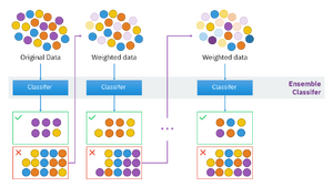
There are many boosting algorithms. The original ones, proposed by Robert Schapire (a recursive majority gate formulation)[31] and Yoav Freund (boost by majority),[35] were not adaptive and could not take full advantage of the weak learners. Schapire and Freund then developed AdaBoost, an adaptive boosting algorithm that won the prestigious Gödel Prize.
Only algorithms that are provable boosting algorithms in the probably approximately correct learning formulation can accurately be called boosting algorithms. Other algorithms that are similar in spirit to boosting algorithms are sometimes called "leveraging algorithms", although they are also sometimes incorrectly called boosting algorithms.[35]
The main variation between many boosting algorithms is their method of weighting training data points and hypotheses. AdaBoost is very popular and the most significant historically as it was the first algorithm that could adapt to the weak learners. It is often the basis of introductory coverage of boosting in university machine learning courses.[36] There are many more recent algorithms such as LPBoost, TotalBoost, BrownBoost, xgboost, MadaBoost, LogitBoost, and others. Many boosting algorithms fit into the AnyBoost framework,[35] which shows that boosting performs gradient descent in a function space using a convex cost function.
Notes
- Aslam, Javed A.; Popa, Raluca A.; and Rivest, Ronald L. (2007); On Estimating the Size and Confidence of a Statistical Audit, Proceedings of the Electronic Voting Technology Workshop (EVT '07), Boston, MA, August 6, 2007. More generally, when drawing with replacement [math]n[/math] values out of a set of [math]n[/math] (different and equally likely), the expected number of unique draws is [math]n(1 - e^{-n'/n})[/math].
- 2.0 2.1 Breiman, Leo (1996). "Bagging predictors". Machine Learning 24 (2): 123–140. doi:.
- Breiman, Leo (September 1994). "Bagging Predictors". Technical Report. Department of Statistics, University of California Berkeley.
- Sahu, A., Runger, G., Apley, D., Image denoising with a multi-phase kernel principal component approach and an ensemble version, IEEE Applied Imagery Pattern Recognition Workshop, pp.1-7, 2011.
- Shinde, Amit, Anshuman Sahu, Daniel Apley, and George Runger. "Preimages for Variation Patterns from Kernel PCA and Bagging." IIE Transactions, Vol.46, Iss.5, 2014
- 6.0 6.1 6.2 Ho, Tin Kam (1995). Random Decision Forests (PDF). Proceedings of the 3rd International Conference on Document Analysis and Recognition, Montreal, QC, 14–16 August 1995. pp. 278–282. Archived from the original (PDF) on 17 April 2016. Retrieved 5 June 2016.
- 7.0 7.1 Ho, Tin Kam (1998). "The Random Subspace Method for Constructing Decision Forests". IEEE Transactions on Pattern Analysis and Machine Intelligence 20 (8): 832–844. doi:.
- 8.0 8.1 "Role of Data Analytics in Infrastructure Asset Management: Overcoming Data Size and Quality Problems" (2020-06-01). Journal of Transportation Engineering, Part B: Pavements 146 (2): 04020022. doi:.
- "Using Machine Learning to Examine Impact of Type of Performance Indicator on Flexible Pavement Deterioration Modeling" (in en) (2021-02-01). Journal of Infrastructure Systems 27 (2): 04021005. doi:. ISSN 1076-0342.
- Kleinberg, Eugene (1990). "Stochastic Discrimination". Annals of Mathematics and Artificial Intelligence 1 (1–4): 207–239. doi:.
- Kleinberg, Eugene (1996). "An Overtraining-Resistant Stochastic Modeling Method for Pattern Recognition". Annals of Statistics 24 (6): 2319–2349. doi:.
- Kleinberg, Eugene (2000). "On the Algorithmic Implementation of Stochastic Discrimination". IEEE Transactions on PAMI 22 (5): 473–490. doi:.
- 13.0 13.1 Breiman, Leo (2001). "Random Forests". Machine Learning 45 (1): 5–32. doi:. Bibcode: 2001MachL..45....5B.
- 14.0 14.1 Liaw A (16 October 2012). "Documentation for R package randomForest" (PDF). Retrieved 15 March 2013.
- U.S. trademark registration number 3185828, registered 2006/12/19.
- "RANDOM FORESTS Trademark of Health Care Productivity, Inc. - Registration Number 3185828 - Serial Number 78642027 :: Justia Trademarks".
- "Shape quantization and recognition with randomized trees" (1997). Neural Computation 9 (7): 1545–1588. doi:.
- 18.0 18.1 18.2 18.3 18.4 Hastie, Trevor; Tibshirani, Robert; Friedman, Jerome (2008). The Elements of Statistical Learning (2nd ed.). Springer. ISBN 0-387-95284-5.
- Gareth James; Daniela Witten; Trevor Hastie; Robert Tibshirani (2013). An Introduction to Statistical Learning. Springer. pp. 316–321.
- Ho, Tin Kam (2002). "A Data Complexity Analysis of Comparative Advantages of Decision Forest Constructors". Pattern Analysis and Applications 5 (2): 102–112. doi:.
- "Reinforcement Learning Trees" (2015). Journal of the American Statistical Association 110 (512): 1770–1784. doi:. PMID 26903687.
- Deng, H.; Runger, G.; Tuv, E. (2011). Bias of importance measures for multi-valued attributes and solutions. Proceedings of the 21st International Conference on Artificial Neural Networks (ICANN). pp. 293–300.
- "Permutation importance: a corrected feature importance measure" (May 2010). Bioinformatics 26 (10): 1340–7. doi:. PMID 20385727.
- "Unbiased split selection for classification trees based on the Gini index" (2007). Computational Statistics & Data Analysis 52: 483–501. doi:.
- "Cross-Validated Variable Selection in Tree-Based Methods Improves Predictive Performance" (2017). IEEE Transactions on Pattern Analysis and Machine Intelligence 39 (11): 2142–2153. doi:. PMID 28114007.
- "Classification with correlated features: unreliability of feature ranking and solutions" (July 2011). Bioinformatics 27 (14): 1986–94. doi:. PMID 21576180.
- Leo Breiman (1996). "BIAS, VARIANCE, AND ARCING CLASSIFIERS" (PDF). TECHNICAL REPORT. Archived from the original (PDF) on 2015-01-19. Retrieved 19 January 2015.
Arcing [Boosting] is more successful than bagging in variance reduction
- Zhou Zhi-Hua (2012). Ensemble Methods: Foundations and Algorithms. Chapman and Hall/CRC. p. 23. ISBN 978-1439830031.
The term boosting refers to a family of algorithms that are able to convert weak learners to strong learners
- 29.0 29.1 Michael Kearns(1988); Thoughts on Hypothesis Boosting, Unpublished manuscript (Machine Learning class project, December 1988)
- Michael Kearns; Leslie Valiant (1989). Template:Sic limitations on learning Boolean formulae and finite automata. Symposium on Theory of Computing. 21. ACM. pp. 433–444. doi:10.1145/73007.73049. ISBN 978-0897913072. S2CID 536357.
- 31.0 31.1 Schapire, Robert E. (1990). "The Strength of Weak Learnability". Machine Learning 5 (2): 197–227. doi:.
- Leo Breiman (1998). "Arcing classifier (with discussion and a rejoinder by the author)". Ann. Stat. 26 (3): 801–849. doi:. “Schapire (1990) proved that boosting is possible. (Page 823)”
- Yoav Freund and Robert E. Schapire (1997); A Decision-Theoretic Generalization of On-Line Learning and an Application to Boosting, Journal of Computer and System Sciences, 55(1):119-139
- Leo Breiman (1998); Arcing Classifier (with Discussion and a Rejoinder by the Author), Annals of Statistics, vol. 26, no. 3, pp. 801-849: "The concept of weak learning was introduced by Kearns and Valiant (1988, 1989), who left open the question of whether weak and strong learnability are equivalent. The question was termed the boosting problem since [a solution must] boost the low accuracy of a weak learner to the high accuracy of a strong learner. Schapire (1990) proved that boosting is possible. A boosting algorithm is a method that takes a weak learner and converts it into a strong learner. Freund and Schapire (1997) proved that an algorithm similar to arc-fs is boosting.
- 35.0 35.1 35.2 Llew Mason, Jonathan Baxter, Peter Bartlett, and Marcus Frean (2000); Boosting Algorithms as Gradient Descent, in S. A. Solla, T. K. Leen, and K.-R. Muller, editors, Advances in Neural Information Processing Systems 12, pp. 512-518, MIT Press
- Emer, Eric. "Boosting (AdaBoost algorithm)" (PDF). MIT. Retrieved 2018-10-10.
Further Reading
- Breiman, Leo (1996). "Bagging predictors". Machine Learning 24 (2): 123–140. doi:.
- Alfaro, E., Gámez, M. and García, N. (2012). "adabag: An R package for classification with AdaBoost.M1, AdaBoost-SAMME and Bagging".
- Kotsiantis, Sotiris (2014). "Bagging and boosting variants for handling classifications problems: a survey". Knowledge Eng. Review 29 (1): 78–100. doi:.
- Boehmke, Bradley; Greenwell, Brandon (2019). "Bagging". Hands-On Machine Learning with R. Chapman & Hall. pp. 191–202. ISBN 978-1-138-49568-5.
References
- Wikipedia contributors. "Bootstrap aggregating". Wikipedia. Wikipedia. Retrieved 17 August 2022.
- Wikipedia contributors. "Boosting (machine learning)". Wikipedia. Wikipedia. Retrieved 17 August 2022.
- Wikipedia contributors. "Random forest". Wikipedia. Wikipedia. Retrieved 17 August 2022.