A Basic Setup

[math] \newcommand{\indep}[0]{\perp\!\!\!\perp} \newcommand{\dpartial}[2]{\frac{\partial #1}{\partial #2}} \newcommand{\abs}[1]{\left| #1 \right|} \newcommand\autoop{\left(} \newcommand\autocp{\right)} \newcommand\autoob{\left[} \newcommand\autocb{\right]} \newcommand{\vecbr}[1]{\langle #1 \rangle} \newcommand{\ui}{\hat{\imath}} \newcommand{\uj}{\hat{\jmath}} \newcommand{\uk}{\hat{k}} \newcommand{\V}{\vec{V}} \newcommand{\half}[1]{\frac{#1}{2}} \newcommand{\recip}[1]{\frac{1}{#1}} \newcommand{\invsqrt}[1]{\recip{\sqrt{#1}}} \newcommand{\halfpi}{\half{\pi}} \newcommand{\windbar}[2]{\Big|_{#1}^{#2}} \newcommand{\rightinfwindbar}[0]{\Big|_{0}^\infty} \newcommand{\leftinfwindbar}[0]{\Big|_{-\infty}^0} \newcommand{\state}[1]{\large\protect\textcircled{\textbf{\small#1}}} \newcommand{\shrule}{\\ \centerline{\rule{13cm}{0.4pt}}} \newcommand{\tbra}[1]{$\bra{#1}$} \newcommand{\tket}[1]{$\ket{#1}$} \newcommand{\tbraket}[2]{$\braket{1}{2}$} \newcommand{\infint}[0]{\int_{-\infty}^{\infty}} \newcommand{\rightinfint}[0]{\int_0^\infty} \newcommand{\leftinfint}[0]{\int_{-\infty}^0} \newcommand{\wavefuncint}[1]{\infint|#1|^2} \newcommand{\ham}[0]{\hat{H}} \newcommand{\mathds}{\mathbb}[/math]

Correlation, Independence and Causation

Two random variables, [math]u[/math] and [math]v[/math], are independent if and only if

[[math]] \begin{align} p(u, v) = p(u) p(v). \end{align} [[/math]]

That is, the probability of [math]u[/math] taking a certain value is not affected by that of [math]v[/math] taking another value. We say [math]u[/math] and [math]v[/math] are dependent upon each other when the condition above does not hold. In everyday life, we often confuse dependence with correlation, where two variables are correlated if and only if

[[math]] \begin{align} \mathrm{cov}(u,v) = \mathbb{E}\left[ (u - \mu_u) (v - \mu_v) \right] \gt 0, \end{align} [[/math]]

where [math]\mu_u = \mathbb{E}[u][/math] and [math]\mu_v = \mathbb{E}[v][/math]. When this covariance is [math]0[/math], we say these two variables are uncorrelated. Despite our everyday confusion, these two quantities are only related and not equivalent. When two variables are independent, they are also uncorrelated, but when two variables are uncorrelated, they may not be independent. Furthermore, it turned out these two quantities are also only remotely related to the existence/lack of causation between two variables. You must have heard of the statement “correlation does not imply causation.” There are two sides to this statement. First, the existence of correlation between two variables does not imply that there exists a causal relationship between these two variables. An extreme example of this is tautology; if the relationship between [math]u[/math] and [math]v[/math] is identity, there is no causal relationship but the correlation between these two is maximal. Second, the lack of correlation does not imply the lack of causation. This is the more important aspect of this statement. Even if there is no correlation between two variables, there could be a causal mechanism behind these two variables. Although it is a degenerate case, consider the following structural causal model:

[[math]] \begin{align} &a \leftarrow -u + \epsilon_a \\ &b \leftarrow +u + \epsilon_b \\ &v \leftarrow a + b + \epsilon_v. \end{align} [[/math]]

The value of [math]v[/math] is caused by [math]u[/math] via two paths; [math]u \to a \to v[/math] and [math]u \to b \to v[/math], but these paths cancel each other. If we only observe [math](u,v)[/math] pairs, it is easy to see that they are uncorrelated, since [math]v[/math] is constant. We will have more discussion later in the semester, but it is good time for you to pause and think whether these two paths matter, since they cancel each other. Consider as another example the following structural causal model:

[[math]] \begin{align} &z \leftarrow \epsilon_z \\ &u \leftarrow 0.2 z + \sqrt{1.04} \epsilon_u \\ &v \leftarrow 0.1 u - 0.5 z + 0.1 \epsilon_v, \end{align} [[/math]]

where [math]\epsilon_z[/math], [math]\epsilon_u[/math] and [math]\epsilon_v[/math] are all standard Normal variables. Again, the structural causal model clearly indicates that [math]u[/math] causally affects [math]v[/math] via [math]0.1 u[/math], but the correlation between [math]u[/math] and [math]v[/math] is [math]0[/math] when we consider those two variables alone (that is, after marginalizing out [math]z[/math]). This second observation applies equally to independence. That is, the independence between two variables does not imply the lack of a causal mechanism between two variables. The examples above apply here equally, as two uncorrelated Normal variables are also independent. This observation connects to an earlier observation that there are potentially many data generating processes that give rise to the same conditional distribution between two sets of variables. Here as well, the independence or correlatedness of two variables may map to many different generating processes that encode different causal mechanisms behind these variables. In other words, we cannot determine the causal relationship between two variables (without loss of generality) without predefining the underlying generating process (in terms of either the probabilistic graphical model or equivalently the structural causal model.) In other words, we must consider both variables of interest and the associated data generating model in order to determine whether there exists a causal relationship between these variables and what that relationship is.

Confounders, Colliders and Mediators

Let us consider a simple scenario where there are only three variables; [math]u[/math], [math]v[/math] and [math]w[/math]. We are primarily interested in the relationship between the first two variables; [math]u[/math] and [math]v[/math]. We will consider various ways in which these three variables are connected with each other and how such wiring affects the relationship between [math]u[/math] and [math]v[/math].

Directly connected. Consider the following probabilistic graphical model.

[math]w[/math] does not affect either [math]u[/math] nor [math]v[/math], while [math]u[/math] directly causes [math]v[/math]. In this case, the causal relationship between [math]u[/math] and [math]v[/math] is clear. If we perturb [math]u[/math], it will affect [math]v[/math], according to the conditional distribution [math]p_v(v | u)[/math]. This tells us that we can ignore any node in a probabilistic graphical model that is not connected to any variable of interest.

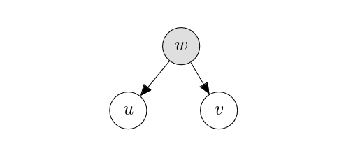
An observed confounder. Consider the following probabilistic graphical model, where [math]w[/math] is shaded, which indicates that [math]w[/math] is observed.

In this graph, the value/distribution of [math]u[/math] and that of [math]v[/math] are both determined individually already because we have observed [math]w[/math]. This corresponds to the definition of conditional independence;

[[math]] \begin{align} p(u,v |w) = p(u|w) p(v|w). \end{align} [[/math]]

Because the edge is directed from [math]w[/math] to [math]u[/math], perturbing [math]u[/math] does not change the observed value of [math]w[/math]. The same applies to [math]v[/math] as well, since perturbing [math]v[/math] does not affect [math]u[/math], since this path between [math]u[/math] and [math]v[/math] via [math]w[/math] is blocked by observing [math]w[/math].

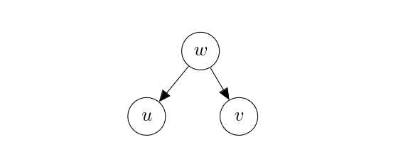
An unobserved confounder. Consider the case where [math]w[/math] was not observed.

We first notice that in general

[[math]] \begin{align} p(u,v) = \int_w p(u|w)p(v|w)p(w) \mathrm{d}w \neq q(u)q(v), \end{align} [[/math]]

implying that [math]u[/math] and [math]v[/math] are not independent, unlike when [math]w[/math] was not observed. In other words, [math]u[/math] and [math]v[/math] are not conditionally independent given [math]w[/math]. Perturbing [math]u[/math] however still does not affect [math]v[/math], since the value of [math]w[/math] is not determined by the value of [math]u[/math] according to the corresponding causal structural model. That is, [math]u[/math] does not affect [math]v[/math] causally (and vice versa.) This is the case where the independence and causality start to deviate from each other; [math]u[/math] and [math]v[/math] are not independent but each is not the cause of the other. Analogous to the former case of the observed [math]w[/math], where we say the path [math]u \leftarrow w \to v[/math] was closed, we say that the same path is open in this latter case. Because of this effect [math]w[/math] has, we call it a confounder. The existence of a confounder [math]w[/math] makes it difficult to tell whether the dependence between two variables we see is due to a causal relationship between these variables. [math]w[/math] confounds this analysis.

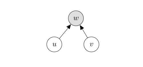
An observed collider. Consider the following graph where the arrows are flipped.

In general,

[[math]] \begin{align} p(u,v | w) = \frac{p(w|u, v) p(u) p(v)} {\int \int p(w|u, v) p(u) p(v) \mathrm{d}u \mathrm{d}v} \neq q(u) q(v), \end{align} [[/math]]

which means that [math]u[/math] and [math]v[/math] are not independent conditioned on [math]w[/math]. This is sometimes called the explaining-away effect, because observing [math]w[/math] explains away one of two potential causes behind [math]w[/math]. Although [math]u[/math] and [math]v[/math] are not independent in this case, there is no causal relationship between [math]u[/math] and [math]v[/math]. [math]w[/math] is where the causal effects of [math]u[/math] and [math]v[/math] collide with each other (hence, [math]w[/math] is a collider) and does not pass along the causal effect between [math]u[/math] and [math]v[/math]. Similarly to the case of an unobserved confounder above, this is one of those cases where independence does not imply causation. We say that the path [math]u \to w \leftarrow v[/math] is open.

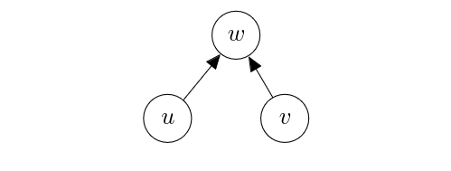
An unobserved collider. Consider the case where the collider [math]w[/math] is not observed.

By construction, [math]u[/math] and [math]v[/math] are independent, as

[[math]] \begin{align} p(u,v) = \int p(u) p(v) p(w|u,v) \mathrm{d}w = p(u) p(v) \int p(w | u, v) \mathrm{d}w = p(u) p(v). \end{align} [[/math]]

Just like before, neither [math]u[/math] or [math]v[/math] is the cause of the other. This path is closed.

An observed mediator. Consider the case where there is an intermediate variable between [math]u[/math] and [math]v[/math]:

Because

[[math]] \begin{align} p(u,v | w) = p(u) p(w|u) p(v|w) = q(u|w) q(v|w) \end{align} [[/math]]

[math]u[/math] and [math]v[/math] are independent conditioned on [math]w[/math]. However, perturbing [math]u[/math] does not affect [math]v[/math], since the value of [math]w[/math] is observed (that is, fixed.) We say that [math]u \to w \to v[/math] is closed in this case, and independence implies the lack of causality.

An unobserved mediator. What if [math]w[/math] is not observed, as below?

It is then clear that [math]u[/math] and [math]v[/math] are not independent, since

[[math]] \begin{align} p(u,v) = \int p(u) p(w|u) p(v|w) \mathrm{d} w = p(u) \int p(w|u) p(v|w) \mathrm{d} w = p(u) q(v|u). \end{align} [[/math]]

Perturbing [math]u[/math] will change the distribution/value of [math]w[/math] which will consequently affect that of [math]v[/math], meaning that [math]u[/math] causally affects [math]v[/math]. This effect is mediated by [math]w[/math], and hence we call [math]w[/math] a mediator.

Dependence and Causation

We can chain the rules that were defined between three variables; [math]u[/math], [math]v[/math] and [math]w[/math], in order to determine the dependence between two nodes, [math]u[/math] and [math]v[/math], within any arbitrary probabilistic graphical model given a set [math]Z[/math] of observed nodes. This procedure is called D-separation, and it tells us two things. First, we can check whether

[[math]] \begin{align} u \indep_Z v. \end{align} [[/math]]

More importantly, however, we get all open paths between [math]u[/math] and [math]v[/math]. These open paths are conduits that carry statistical dependence between [math]u[/math] and [math]v[/math] regardless of whether there is a causal path between [math]u[/math] and [math]v[/math], where we define a causal path as an open directed path between [math]u[/math] and [math]v[/math]. Dependencies arising from open, non-causal paths are often casually referred to as ‘spurious correlation’ or ‘spurious dependency’. When we are performing causal inference for the purpose of designing a causal intervention in the future, it is imperative to dissect out these spurious correlations and identify true causal relationship between [math]u[/math] and [math]v[/math]. It is however unclear whether we want to remove all spurious dependencies or whether we should only remove spurious dependencies that are unstable, when it comes to prediction in machine learning. We will discuss more about this contention later in the course. In this course, we do not go deeper into D-separation. We instead stick to a simple setting where there are only three or four variables, so that we can readily identify all open paths and determine which are causal and which others are spurious.

Causal Effects

We have so far avoided defining more carefully what it means for a node [math]u[/math] to effect another node [math]v[/math] causally. Instead, we simply said [math]u[/math] effects [math]v[/math] causally if there is a directed path from [math]u[/math] to [math]v[/math] under the underlying data generating process. This is however unsatisfactory, as there are loopholes in this approach. The most obvious one is that some of those directed edges may correspond to a constant function. For instance, an extreme case is where the structural causal model is

[[math]] \begin{align} &a \leftarrow f_a(u, \epsilon_a) \\ &v \leftarrow f_v(a, \epsilon_v), \end{align} [[/math]]

where [math]f_a(\cdot) = 0[/math]. In this case, the edge from [math]u[/math] to [math]a[/math] is effectively non-existent, although we wrote it as if it existed. Rather, we want to define a causal effect of [math]u[/math] on [math]v[/math] by thinking of how perturbation on [math]u[/math] propagates over the data generating process and arrives at [math]v[/math]. More specifically, we consider forcefully setting the variable [math]u[/math] (the cause variable) to an arbitrary value [math]\hat{u}[/math]. This corresponds to replacing the following line in the structural causal model [math]G=(V,F,U)[/math]

[[math]] \begin{align} u \leftarrow f_u(\mathrm{pa}(u), \epsilon_u) \end{align} [[/math]]

with

[[math]] \begin{align} u \leftarrow \hat{u}. \end{align} [[/math]]

[math]\hat{u}[/math] can be a constant or can also be a random variable as long as it is not dependent on any other variables in the structural causal model. Once this replacement is done, we run this modified structural causal model [math]\overline{G}(\hat{u})=(\overline{V},\overline{F},U)[/math] in order to compute the following expected outcome:

[[math]] \begin{align} \mathbb{E}_{U}[v_{\overline{\mathcal{G}}(\hat{u})}], \end{align} [[/math]]

where [math]U[/math] is a set of exogenous factors (e.g. noise.) If [math]u[/math] does not affect [math]v[/math] causally, this expected outcome would not change (much) regardless of the choice of [math]\hat{u}[/math]. As an example, assume [math]u[/math] can take either [math]0[/math] or [math]1[/math], as in treated or placebo. We then check the expected treatment effect on the outcome [math]v[/math] by

[[math]] \begin{align} \mathbb{E}_{U}[v_{\overline{\mathcal{G}}(\hat{u}=1)}] - \mathbb{E}_{U}[v_{\overline{\mathcal{G}}(\hat{u}=0)}]. \end{align} [[/math]]

We would want this quantity to be positive and large to know that the treatment has a positive causal effect on the outcome. This procedure of forcefully setting a variable to a particular value is called a [math]\mathrm{do}[/math] operator. The impact of [math]\mathrm{do}[/math] is more starkly demonstrated if we consider a probabilistic graphical model rather than a structural causal model. Let [math]p_u(u | \mathrm{pa}(u))[/math] be the conditional distribution over [math]u[/math] in a probabilistic graphical model [math]G=(V,E,P)[/math]. We construct a so-called interventional distribution as

[[math]] \begin{align} p(v | \mathrm{do}(u = \hat{u})), \end{align} [[/math]]

which states that we are now forcefully setting [math]u[/math] to [math]\hat{u}[/math] instead of letting it be a sample drawn from the conditional distribution [math]p_u(u | \mathrm{pa}(u))[/math]. That is, instead of

[[math]] \begin{align} u \sim u | \mathrm{pa}(u), \end{align} [[/math]]

we do

[[math]] \begin{align} u \leftarrow \hat{u}. \end{align} [[/math]]

In other words, we replace the conditional probability [math]p_u(u | \mathrm{pa}(u))[/math] with

[[math]] \begin{align} p_u(u | \mathrm{pa}(u)) = \delta(u - \hat{u}), \end{align} [[/math]]

where [math]\delta[/math] is a Dirac measure, or replace all occurrences of [math]u[/math] in the conditional probabilities of [math]\mathrm{child}(u)[/math] with a constant [math]\hat{u}[/math], where

[[math]] \begin{align} \mathrm{child}(u) = \left\{ u' \in V | (u, v') \in E \right\}. \end{align} [[/math]]

As a consequence, in the new modified graph [math]\overline{G}[/math], there is no edge coming into [math]u[/math] (or [math]\hat{u}[/math]) anymore, i.e., [math]\mathrm{pa}(u) = \emptyset[/math]. [math]u[/math] is now independent of all the other nodes a priori. Because [math]\mathrm{do}[/math] modifies the underlying data generating process, [math]p(v|u=\hat{u}; G)[/math] and [math]p(v|\mathrm{do}(u=\hat{u}); G) = p(v|u=\hat{u}; \overline{G})[/math] differ from each other. This difference signifies the separation between statistical and causal quantities. We consider this separation in some minimal cases.

Case Studies

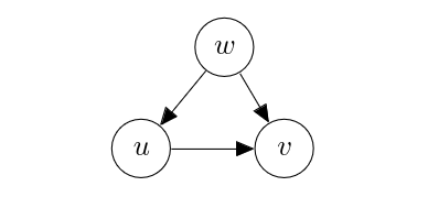
An unobserved confounder and a direct connection. Consider the case where [math]w[/math] was not observed.

Under this graph [math]G[/math],

[[math]] \begin{align} p_G(v|u=\hat{u}) = \frac{\sum_{w} p(w) p(\hat{u}|w) p(v|\hat{u},w)}{p(\hat{u})} = \mathbb{E}_w \left[ \frac{p(\hat{u}|w)}{p(\hat{u})} p(v| \hat{u}, w) \right], \end{align} [[/math]]

from which we see that there are two open paths between [math]v[/math] and [math]u[/math]:

• [math]u \to v[/math]: a direct path;
• [math]u \leftarrow w \to v[/math]: an indirect path via the unobserved confounder.

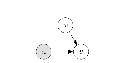
The statistical dependence between [math]u[/math] and [math]v[/math] flows through both of these paths, while the causal effect of [math]u[/math] and [math]v[/math] only flows through the direct path [math]u \to v[/math]. The application of [math]\mathrm{do}(u = \hat{u})[/math] in this case would severe the edge from [math]w[/math] to [math]u[/math], as in

Under this modified graph [math]\overline{G}[/math],

[[math]] \begin{align} p_G(v | \mathrm{do}(u = \hat{u})) &= p_{\tilde{G}}(v | u=\hat{u}) = \frac{1}{q(\hat{u})}\sum_w p(w) q(\hat{u}) p(v | \hat{u}, w) \\ &= \sum_w p(w) p(v | \hat{u}, w) = \mathbb{E}_w \left[ p(v | \hat{u}, w) \right] , \end{align} [[/math]]

where we use [math]q(\hat{u})[/math] to signify that this is not the same as [math]p(\hat{u})[/math] above. The first one [math]p_G(v | u = \hat{u})[/math] is a statistical quantity, and we call it a conditional probability. The latter [math]p_G(v | \mathrm{do}(u = \hat{u}))[/math] is instead a causal quantity, and we call it an interventional probability. Comparing these two quantities, [math]p_G(v | u = \hat{u})[/math] and [math]p_G(v | \mathrm{do}(u = \hat{u}))[/math], the main difference is the multiplicative factor [math]\frac{p(\hat{u}|w)}{p(\hat{u})}[/math] inside the expectation. The numerator [math]p(\hat{u}|w)[/math] tells us how likely this treatment [math]\hat{u}[/math] was given under [math]w[/math], while the denominator [math]p(\hat{u})[/math] tells us how likely the treatment [math]\hat{u}[/math] was given overall. In other words, we upweight the impact of [math]\hat{u}[/math] and [math]w[/math] if [math]\hat{u}[/math] was more probable under [math]w[/math] than overall. This observation will allow us to convert between these two quantities later.

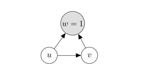
An observed collider and a direct connection. Let us flip the edges from [math]w[/math] so that those edges are directed toward [math]w[/math]. We further assume that we always observe [math]w[/math] to be a constant ([math]1[/math]).

The [math]\mathrm{do}[/math] operator on [math]u[/math] does not alter the graph above. This means that the conditional probability and interventional probability coincide with each other in this case, conditioned on observing [math]w=1[/math]. This however does not mean that the conditional probability [math]p(v|u=\hat{u},w=1)[/math], or equivalently the interventional probability [math]p(v|\mathrm{do}(u=\hat{u}),w=1)[/math], measures the causal effect of [math]u[/math] on [math]v[/math] alone. As we saw before and also can see below, there are two open paths, [math]u \to v[/math] and [math]u \leftarrow w \to v[/math], between [math]u[/math] and [math]v[/math] through which the dependence between [math]u[/math] and [math]v[/math] flows:

[[math]] \begin{align} p(v | u, w=1) = \frac{\cancel{p(u)} p(v | u) p(w=1|u, v)}{\sum_{v'} \cancel{p(u)} p(v'| u) p(w=1|u, v')}. \end{align} [[/math]]

We must then wonder whether we can separate out these two paths from each other. It turned out unfortunately that this is not possible in this scenario, because we need the cases of [math]w \neq 1[/math] (e.g. [math]w=0[/math]) for this separation. If you recall how we can draw samples from a probabilistic graphical model while conditioning some variables to take particular values, it was all about selecting a subset of samples drawn from the same graph without any observed variables. This selection effectively prevents us from figuring out the effect of [math]u[/math] on [math]v[/math] via [math]w[/math]. We will have more discussion on this topic later in the semester in the context of invariant prediction. Because of this inherent challenge, that may not even be addressable in many cases, we will largely stick to the case of having a confounder in this semester.

Summary

In this chapter, we have learned about the following topics:

• How to represent a data generating process: a probabilistic graphical model vs. a structural causal model;
• How to read out various distributions from a data generating process: ancestral sampling and Bayes' rule;
• The effect of confounders, colliders and mediators on independence;
• Causal dependency vs. spurious dependency;
• The [math]\mathrm{do}[/math] operator.

General references

Cho, Kyunghyun (2024). "A Brief Introduction to Causal Inference in Machine Learning". arXiv:2405.08793 [cs.LG].