The figure below shows the cumulative distribution function of a random variable, [math]X[/math].

Calculate [math]\operatorname{E}(X)[/math].

• 0.00
• 0.50
• 1.00
• 1.25
• 2.50

Copyright 2023. The Society of Actuaries, Schaumburg, Illinois. Reproduced with permission.

Solution: D

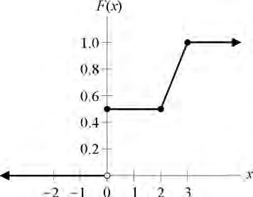
The distribution function plot shows that X has a point mass at 0 with probability 0.5. From 2 to 3 it has a continuous distribution. The density function is the derivative, which is the constant (1– 0.5)/(3 – 2) = 0.5. The expected value is 0(0.5) plus the integral from 2 to 3 of 0.5x. The integral evaluates to 1.25, which is the answer. Alternatively, this is a 50-50 mixture of a point mass at 0 and a uniform(2,3) distribution. The mean is 0.5(0) + 0.5(2.5) = 1.25.

Copyright 2023. The Society of Actuaries, Schaumburg, Illinois. Reproduced with permission.