Causal Quantities of Interest

[math] \newcommand{\indep}[0]{\ensuremath{\perp\!\!\!\perp}} \newcommand{\dpartial}[2]{\frac{\partial #1}{\partial #2}} \newcommand{\abs}[1]{\left| #1 \right|} \newcommand\autoop{\left(} \newcommand\autocp{\right)} \newcommand\autoob{\left[} \newcommand\autocb{\right]} \newcommand{\vecbr}[1]{\langle #1 \rangle} \newcommand{\ui}{\hat{\imath}} \newcommand{\uj}{\hat{\jmath}} \newcommand{\uk}{\hat{k}} \newcommand{\V}{\vec{V}} \newcommand{\half}[1]{\frac{#1}{2}} \newcommand{\recip}[1]{\frac{1}{#1}} \newcommand{\invsqrt}[1]{\recip{\sqrt{#1}}} \newcommand{\halfpi}{\half{\pi}} \newcommand{\windbar}[2]{\Big|_{#1}^{#2}} \newcommand{\rightinfwindbar}[0]{\Big|_{0}^\infty} \newcommand{\leftinfwindbar}[0]{\Big|_{-\infty}^0} \newcommand{\state}[1]{\large\protect\textcircled{\textbf{\small#1}}} \newcommand{\shrule}{\\ \centerline{\rule{13cm}{0.4pt}}} \newcommand{\tbra}[1]{$\bra{#1}$} \newcommand{\tket}[1]{$\ket{#1}$} \newcommand{\tbraket}[2]{$\braket{1}{2}$} \newcommand{\infint}[0]{\int_{-\infty}^{\infty}} \newcommand{\rightinfint}[0]{\int_0^\infty} \newcommand{\leftinfint}[0]{\int_{-\infty}^0} \newcommand{\wavefuncint}[1]{\infint|#1|^2} \newcommand{\ham}[0]{\hat{H}} \newcommand{\mathds}{\mathbb}[/math]

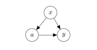
In this chapter, we assume the following graph [math]G[/math]. We use [math]a[/math], [math]y[/math] and [math]x[/math], instead of [math]u[/math], [math]v[/math] and [math]w[/math], to denote the action/treatment, the outcome and the covariate, respectively. The covariate [math]x[/math] is a confounder in this case, and it may or may not observed, depending on the situation.

An example case corresponding to this graph is vaccination.

• [math]a[/math]: is the individual vaccinated?
• [math]y[/math]: has the individual been infected by the target infectious disease with symptoms, within 6 months of vaccine administration?
• [math]x[/math]: the underlying health condition of the individual.

The edge [math]x \to a[/math] is understandable, since we often cannot vaccinate an individual with an active underlying health condition. The edge [math]x \to y[/math] is also understandable, since healthy individuals may contract the disease without any symptoms, while immunocompromised individuals for instance may show a greater degree of symptoms with a higher chance. The edge [math]a \to y[/math] is also reasonable, as the vaccine must have been developed with the target infectious disease as its goal. In other words, this graphs encodes our structural prior about vaccination. With this graph that encodes the reasonable data generating process, causal inference then refers to figuring out the degree of the causal effect of [math]a[/math] on [math]y[/math].

In this particular case, we are interested in a number of causal quantities. The most basic and perhaps most important one is whether the treament is effective (i.e., results in a positive outcome) generally. This corresponds to checking whether [math]\mathbb{E}\left[y | \mathrm{do}(a=1)\right] \gt \mathbb{E}\left[y | \mathrm{do}(a=0)\right][/math], or equivalently computing

[[math]] \begin{align} \mathrm{ATE} = \mathbb{E}\left[y | \mathrm{do}(a=1)\right] - \mathbb{E}\left[y | \mathrm{do}(a=0)\right], \end{align} [[/math]]

where

[[math]] \begin{align} \mathbb{E}\left[y | \mathrm{do}(a=\hat{a})\right] &= \sum_{y} y p(y | \mathrm{do}(a=\hat{a})) \\ &= \sum_{y} y \sum_{x} p(x) p(y|\hat{a}, x) = \sum_{y} y \mathbb{E}_{x \sim p(x)} \left[ p(y|\hat{a}, x) \right]. \end{align} [[/math]]

In words, we average the effect of [math]\hat{a}[/math] on [math]y[/math] over the covariate distribution but the choice of [math]\hat{a}[/math] should not depend on [math]x[/math]. Then, we use this interventional distribution [math]p(y | \mathrm{do}(a=\hat{a}))[/math] to compute the average outcome. We then look at the difference in the average outcome between the treatment and not (placebo), to which we refer as the average treatment effect (ATE). 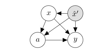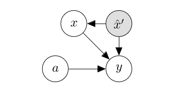It is natural to extend ATE such that we do not marginalize the entire covariate [math]x[/math], but fix some part to a particular value. For instance, we might want to compute ATE but only among people in their twenties. Let us rewrite the covariate [math]x[/math] as a concatenation of [math]x[/math] and [math]x'[/math], where [math]x'[/math] is what we want to condition ATE on. That is, instead of [math]p(y | \mathrm{do}(a=\hat{a}))[/math], we are interested in [math]p(y | \mathrm{do}(a=\hat{a}), x'=\hat{x}')[/math]. This corresponds to first modifying [math]G[/math] into

and then into

We then get the following conditional average treatment effect (CATE):

[[math]] \begin{align} \mathrm{CATE} = \mathbb{E}\left[y | \mathrm{do}(a=1), x'=\hat{x}'\right] - \mathbb{E}\left[y | \mathrm{do}(a=0), x'=\hat{x}'\right], \end{align} [[/math]]

where

[[math]] \begin{align} \mathbb{E}\left[y | \mathrm{do}(a=\hat{a}), x'=\hat{x}'\right] &= \sum_{y} y p(y | \mathrm{do}(a=\hat{a}), x'=\hat{x'}) \\ &= \sum_{y} y \sum_{x} p(x|x') p(y|\hat{a}, x'=\hat{x'}, x) \\ &= \sum_{y} y \mathbb{E}_{x \sim p(x|x')} \left[ p(y|\hat{a}, x'=\hat{x'}, x) \right]. \end{align} [[/math]]

You can see that this is really nothing but ATE conditioned on [math]x'=\hat{x}'[/math]. From these two quantities of interest above, we see that the core question is whether and how to compute the interventional probability of the outcome [math]y[/math] given the intervention on the action [math]a[/math] conditioned on the context [math]x'[/math]. Once we can compute this quantity, we can computer various target quantities under this distribution. We thus do not go deeper into other widely used causal quantities in this course but largely stick to ATE/CATE.

General references

Cho, Kyunghyun (2024). "A Brief Introduction to Causal Inference in Machine Learning". arXiv:2405.08793 [cs.LG].