Riemann Sums and the Trapezoid Rule

[math] \newcommand{\ex}[1]{\item } \newcommand{\sx}{\item} \newcommand{\x}{\sx} \newcommand{\sxlab}[1]{} \newcommand{\xlab}{\sxlab} \newcommand{\prov}[1] {\quad #1} \newcommand{\provx}[1] {\quad \mbox{#1}} \newcommand{\intext}[1]{\quad \mbox{#1} \quad} \newcommand{\R}{\mathrm{\bf R}} \newcommand{\Q}{\mathrm{\bf Q}} \newcommand{\Z}{\mathrm{\bf Z}} \newcommand{\C}{\mathrm{\bf C}} \newcommand{\dt}{\textbf} \newcommand{\goesto}{\rightarrow} \newcommand{\ddxof}[1]{\frac{d #1}{d x}} \newcommand{\ddx}{\frac{d}{dx}} \newcommand{\ddt}{\frac{d}{dt}} \newcommand{\dydx}{\ddxof y} \newcommand{\nxder}[3]{\frac{d^{#1}{#2}}{d{#3}^{#1}}} \newcommand{\deriv}[2]{\frac{d^{#1}{#2}}{dx^{#1}}} \newcommand{\dist}{\mathrm{distance}} \newcommand{\arccot}{\mathrm{arccot\:}} \newcommand{\arccsc}{\mathrm{arccsc\:}} \newcommand{\arcsec}{\mathrm{arcsec\:}} \newcommand{\arctanh}{\mathrm{arctanh\:}} \newcommand{\arcsinh}{\mathrm{arcsinh\:}} \newcommand{\arccosh}{\mathrm{arccosh\:}} \newcommand{\sech}{\mathrm{sech\:}} \newcommand{\csch}{\mathrm{csch\:}} \newcommand{\conj}[1]{\overline{#1}} \newcommand{\mathds}{\mathbb} [/math]

This section is divided into two parts. The first is devoted to an alternative approach to the definite integral, which is useful for many purposes. The second is an application of the first part to the problem of computing definite integrals by numerical approximations. We begin by reviewing briefly the definitions in Section 1 of Chapter 4. If the function [math]f[/math] is bounded on the closed interval [math][a, b][/math], then, for every partition [math]\sigma[/math] of [math][a, b][/math], there are defined an upper sum [math]U_\sigma[/math] and a lower sum [math]L_\sigma[/math], which approximate the definite integral from above and below, respectively. The function [math]f[/math] is defined to be integrable over [math][a, b][/math] if there exists one and only one number, denoted by [math]\int_a^b f[/math], with the property that

[[math]] L_\sigma \leq \int_a^b f \leq U_\tau, [[/math]]

for every pair of partitions [math]\sigma[/math] and [math]\tau[/math] of [math][a, b][/math]. In the alternative description of the integral, the details are similar, but not the same. As above, let [math]\sigma = \{ x_0, . . ., x_n \}[/math] be a partition of [math][a, b][/math], which satisfies the inequalities

[[math]] a = x_0 \leq x_1 \leq ... \leq x_n = b. [[/math]]

In each subinterval [math][x_{i-1}, x_i][/math] we select an arbitrary number, which we shall denote by [math]x_i^{*}[/math]. Then the sum

[[math]] R_\sigma = \sum_{i = 1}^{n} f(x_i^{*})(x_i - x_{i-1}) [[/math]]

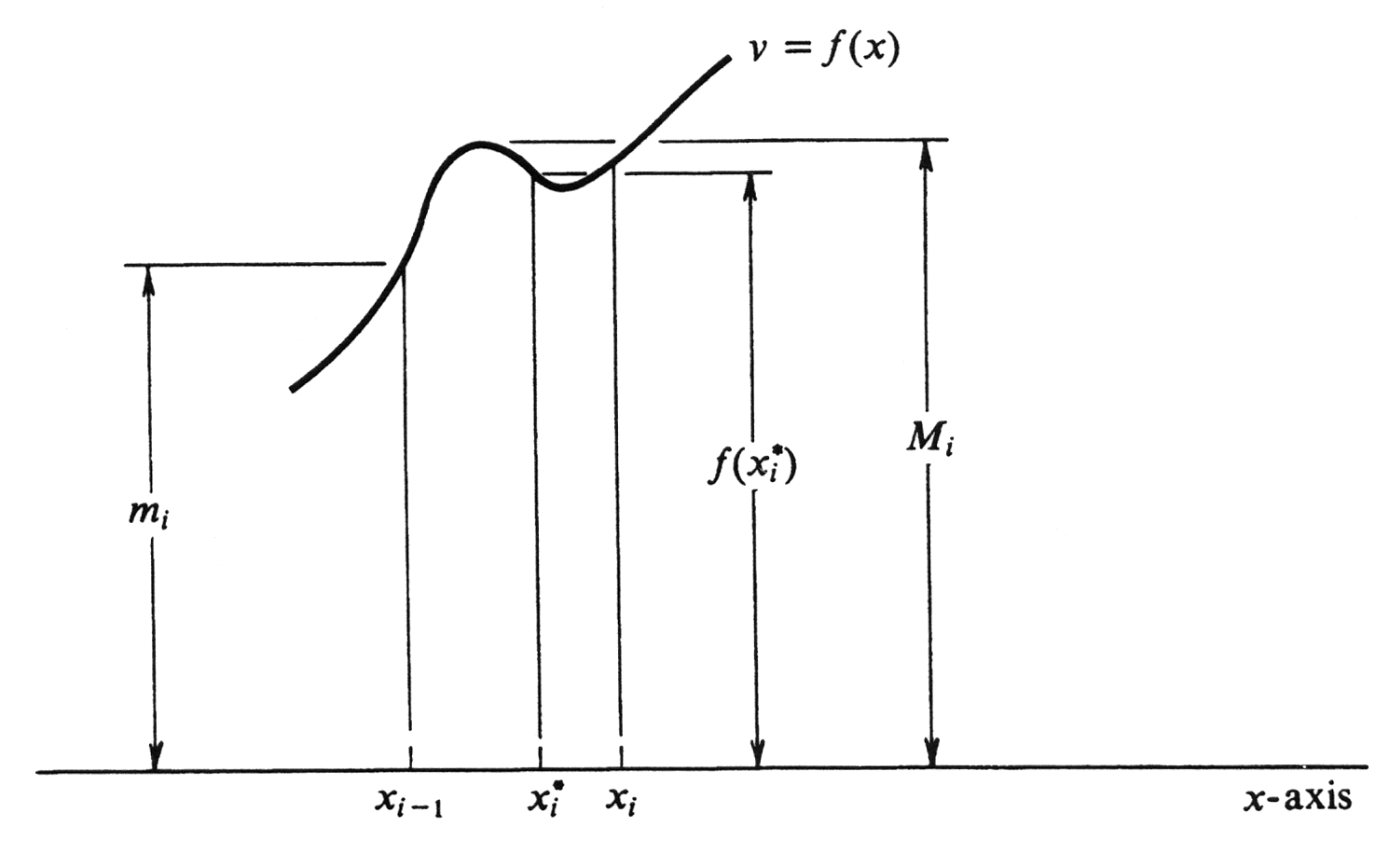
is called a Riemann sum for [math]f[/math] relative to the partition [math]\sigma[/math]. (The name commemorates the great mathematician Bernhard Riemann, 1826-1866.) It is important to realize that since [math]x_i^{*}[/math] may be any number which satisfies [math]x_{i-1} \leq x_i^{*} \leq x_i[/math], there are in general infinitely many Riemann sums [math]R_\sigma[/math] for a given [math]f[/math] and partition [math]\sigma[/math]. However, every [math]R_\sigma[/math] lies between the corresponding upper and lower sums [math]U_\sigma[/math] and [math]L_\sigma[/math]. For, if the least upper bound of the values of [math]f[/math] on [math][x_{i-1}, x_i][/math] is denoted by [math]M_i[/math] and the greatest lower bound by [math]m_i[/math], then [math]f(x_i^{*})[/math] is an intermediate value and

[[math]] m_i \leq f(x_i^{*}) \leq M_i, [[/math]]

as shown in Figure 4. It follows that

[[math]] \sum_{i=1}^n m_{i}(x_i - x_{i - 1}) \leq \sum_{i=1}^n f(x_i^{*})(x_i - x_{i - 1}) \leq \sum_{i=1}^n M_i(x_i - x_{i-1}), [[/math]]

which states that

[[math]] L_\sigma \leq R_\sigma \leq U_\sigma, [[/math]]

for every Riemann sum [math]R_\sigma[/math] for [math]f[/math] relative to [math]\sigma[/math].

File:Guide c5467 scanfig8 4.png

Every Riemann sum is an approximation to the definite integral. By taking partitions which subdivide the interval of integration into smaller and smaller subintervals, we should expect to get better and better approximations to [math]\int_a^b f[/math]. One number which measures the fineness of a given partition [math]\sigma[/math] is the length of the largest subinterval into which [math]\sigma[/math] subdivides [math][a, b][/math]. This number is called the mesh of the partition and is denoted by [math]||\sigma ||[/math]. Thus if [math]\sigma = \{ x_0, ..., x_n \}[/math] is a partition of [math][a, b][/math] with

[[math]] a = x_0 \leq x_1 \leq \cdots \leq x_n = b, [[/math]]

then

[[math]] ||\sigma || = \mbox{maximum} \{ (x_i - x_{i-1}) \} . \;\;\; 1 \leq i \leq n [[/math]]

The following definition states precisely what we mean when we say that the Riemann sums approach a limit as the mesh tends to zero. Let the function [math]f[/math] be bounded on the interval [math][a, b][/math]. We shall write

[[math]] \lim_{||\sigma || \rightarrow 0} R_\sigma = L, [[/math]]

where [math]L[/math] is a real number, if the difference between the number [math]L[/math] and any Riemann sum [math]R_\sigma[/math] for [math]f[/math] is arbitrarily small provided the mesh [math]||\sigma||[/math] is sufficiently small. Stated formally, the limit exists if: For any positive real number [math]\epsilon[/math], there exists a positive real number [math]\delta[/math] such that, if [math]R_\sigma[/math] is any Riemann sum for [math]f[/math] relative to a partition [math]\sigma[/math] of [math][a, b][/math] and if [math]|| \sigma || \lt \delta[/math], then [math] | R_\sigma - L | \lt \epsilon[/math]. The fundamental fact that integrability is equivalent to the existence of the limit of Riemann sums is expressed in the following theorem.

Theorem

Let [math]f[/math] be bounded on [math][a, b][/math]. Then [math]f[/math] is integrable over [math][a, b][/math] if and only if [math]\lim_{|| \sigma || \rightarrow 0} R_\sigma[/math] exists. If this limit exists, then it is equal to [math]\int_a^b f[/math].

The proof is given in Appendix C.

Example Using the fact that the definite integral is the limit of Riemann sums, evaluate

[[math]] \lim_{n \rightarrow \infty} \frac{\sqrt 1 + \sqrt 2 + ... + \sqrt n}{n^{3/2}}. [[/math]]

The numerator of this fraction suggests trying the function [math]f[/math] defined by [math]f(x) = \sqrt x[/math]. If [math] \sigma = \{ x_0, . . ., x_n \}[/math] is the partition of the interval [math][0, 1][/math] into subintervals of length [math]\frac{1}{n}[/math], then

[[math]] \begin{array}{rl} x_0 = 0, \;\;\; x_1 = \frac{1}{n},\;\;\;& x_2 = \frac{2}{n}, ... , x_i = \frac{i}{n},\\ x_i - x_{i-1} = \frac{1}{n},\;\;\;& \;\;\;\mbox{for}\; i = 1, ... , n. \end{array} [[/math]]

In each subinterval [math][x_{i-1}, x_i][/math] we take [math]x_{i}^{*} = x_i[/math]. Then

[[math]] f(x_i^{*}) = f(x_i) = \sqrt {\frac{i}{n}} = \frac{\sqrt i}{\sqrt n}, [[/math]]

and the resulting Riemann sum, denoted by [math]R_n[/math], is given by

[[math]] \begin{eqnarray*} R_n &=& \sum_{i = 1}^{n} f(x_{i}^{*})(x_i - x_{i-1}) = \sum_{i = 1}^{n} \frac{\sqrt i}{\sqrt n} \frac{1}{n} \\ &=& \frac{1}{n^{3/2}} \sum_{i = 1}^{n} \sqrt i \\ &=& \frac{\sqrt 1 + \sqrt 2 + ... + \sqrt n}{n^{3/2}} . \end{eqnarray*} [[/math]]

The function [math]\sqrt x[/math] is continuous and hence integrable over the interval [math][0, 1][/math]. Since [math]|| \sigma || \rightarrow 0[/math] as [math]n \rightarrow \infty[/math], it follows from Theorem (2.1) that

[[math]] \int_a^b f = \int_0^1 \sqrt x dx = \lim_{n \rightarrow \infty} R_n. [[/math]]

Hence

[[math]] \begin{eqnarray*} \lim_{n \rightarrow \infty} \frac{\sqrt 1 + \sqrt 2 + ... + \sqrt n}{n^{3/2}} &=& \int_0^1 \sqrt x dx \\ &=& \frac{2}{3} x^{3/2} \Big|_0^1 = \frac{2}{3}, \end{eqnarray*} [[/math]]

and the problem is solved.

Theorem (2.1) shows that it is immaterial whether we define the definite integral in terms of upper and lower sums (as is done in this book) or as the limit of Riemann sums. Hence there is no logical necessity for introducing the latter at all. However, a striking illustration of the practical use of Riemann sums arises in studying the problem of evaluating definite integrals by numerical methods. In spite of the variety of techniques which exist for finding antiderivatives and the existence of tables of indefinite integrals,there are still many functions for which we cannog find an antiderivative. More often than not, the only way of computing [math]\int_a^b f(x) dx[/math] is by numerical approximation. However, the increasing availability of high-speed computers has placed these methods in an entirely new light. Evaluating [math]\int_a^b f (x) dx[/math] by numerical approximation is no longer to be regarded as a last resort to be used only if all else fails. It is an interesting, instructive, and simple task to write a machine program to do the job, and the hundreds, thousands, or even millions of arithmetic operations which may be needed to obtain the answer to a desired accuracy can be performed by a machine in a matter of seconds or minutes. One of the simplest and best of the techniques of numerical integration is the Trapezoid Rule, which we now describe. Suppose that the function [math]f[/math] is integrable over the interval [math][a, b][/math]. For every positive integer [math]n[/math], let [math]\sigma_n[/math] be the partition which subdivides [math][a, b][/math] into [math]n[/math] subintervals of equal length [math]h[/math]. Thus [math]\sigma_n = \{ x_0, . . ., x_n \}[/math] and

[[math]] h = \frac{b - a}{n} = x_i - x_{i-1}, \;\;\; i = 1, ... , n. [[/math]]

It is convenient to set

[[math]] y_i = f(x_i), \;\;\; i = 0, 1, ... , n. [[/math]]

Then the Riemann sum obtained by choosing [math]x_i^*[/math] to be the left endpoint of each subinterval [math][x_{i-1}, x_i][/math], i.e., by choosing [math]x_{i}^{*} = x_{i-1}[/math], is given by

[[math]] \sum_{i=1}^{n} f (x_{i}^{*})(x_i - x_{i-1}) = \sum_{i=1}^{n} f (x_{i-1})h = h \sum_{i=1}^{n} y_{i-1} . [[/math]]

Similarly, the Riemann sum obtained by choosing [math]x_{i}^{*}[/math] to be the right endpoint, i.e., by taking [math]x_{i}^{*} = x_i[/math], is

[[math]] \sum_{i=1}^{n} f(x_{i}^{*})(x_i - x_{i-1}) = \sum_{i=1}^{n} f(x_i) h = h \sum_{i=1}^{n} y_i . [[/math]]

The approximation to [math]\int_a^b f[/math] prescribed by the Trapezoid Rule, which we denote by [math]T_n[/math] is by definition the average of these two Riemann sums. Thus

[[math]] \begin{equation} \begin{array}{ll} T_n &= \frac{h \sum_{i=1}^{n} y_{i-1} + h \sum_{i=1}^{n} y_i}{2} \\ &= \frac{h}{2} \Bigl( \sum_{i=1}^{n} y_{i - 1} + \sum_{i=1}^{n} y_i \Bigr) . \end{array} \label{eq8.2.1} \end{equation} [[/math]]

The last expression above can be simplified by observing that

[[math]] \sum_{i=1}^{n} y_{i - 1} + \sum_{i=1}^{n} y_i = y_0 + 2\sum_{i=1}^{n-1} y_i + y_n . [[/math]]

Hence

[[math]] \begin{equation} T_n = h(\frac{1}{2} y_0 + \sum_{i=1}^{n-1} y_i + \frac{1}{2}y_n) . \label{eq8.2.2} \end{equation} [[/math]]

We shall express the fact that [math]T_n[/math] is an approximation to the integral [math]\int_a^b f[/math] by writing [math]\int_a^b f \approx T_n[/math]. The Trapezoid Rule then appears as the formula

Theorem

[[math]] \int_a^b f \approx T_n = h (\frac{1}{2}y_0 + y_1 + \cdots + y_{n-1} + \frac{1}{2} y_n) . [[/math]]

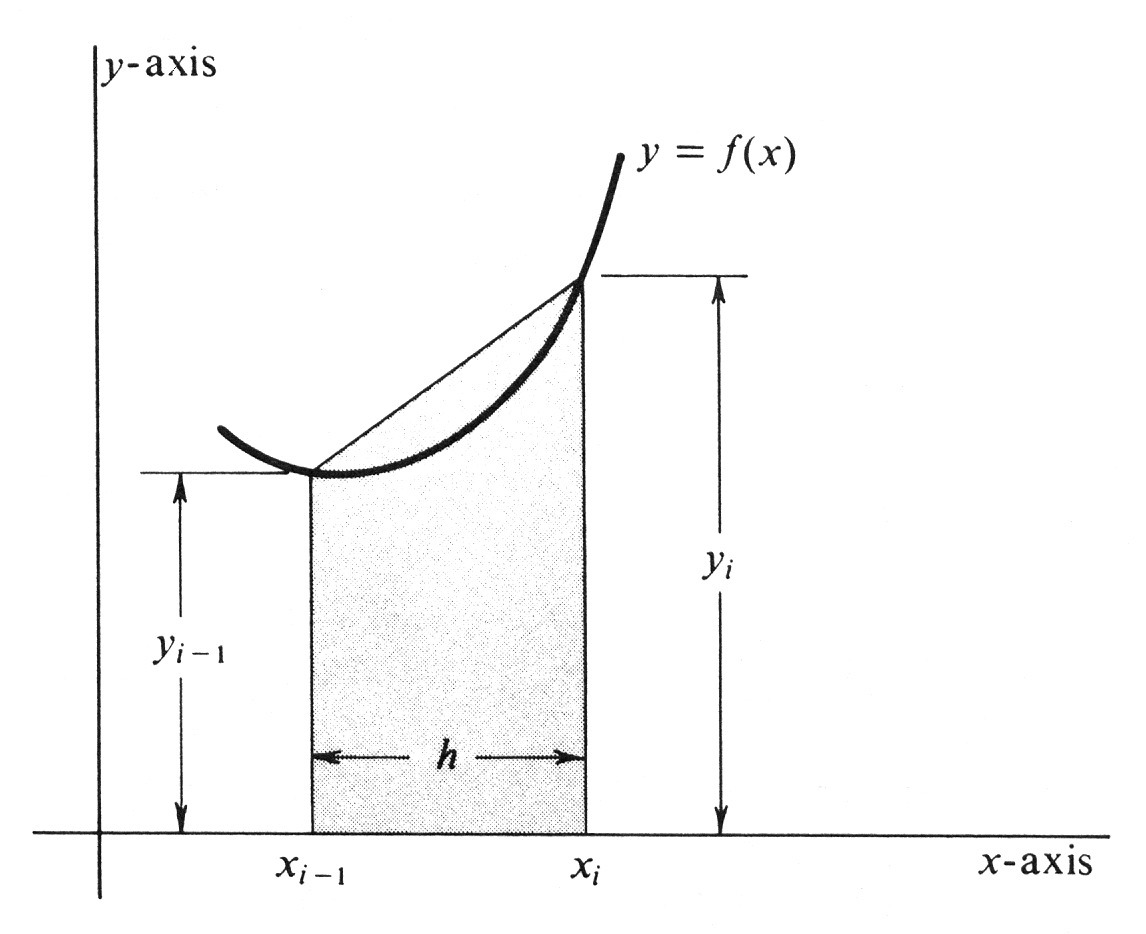
Why is this formula called the Trapezoid Rule? Suppose that [math]f(x) \geq 0[/math] for every [math]x[/math] in [math][a, b][/math], and observe that

[[math]] \int_a^b f = \int_{x_0}^{x_1} f + \int_{x_1}^{x_2} f + \cdots + \int_{x_{n-1}}^{x_n} f. [[/math]]

The area of the shaded trapezoid shown in Figure 5 is an approximation to [math]\int_{x_{i-1}}^{x_i} f[/math]. This trapezoid has bases [math]y_{i-1} = f(x_{i-1})[/math] and [math]y_i = f(x_i)[/math] and altitude [math]h[/math]. By a well-known formula, its area is therefore equal to [math]\frac{h}{2} (y_{i-1} + y_i)[/math]. The integral [math]\int_a^b f[/math] is therefore approximated by the sum of the areas of the trapezoids, which is equal to

[[math]] \sum \frac{h}{2} (y_{i-1} + y_i) = \frac{h}{2} \Bigl( \sum_{i=1}^{n} y_{i -1} + \sum _{i=1}^{n} y_i \Bigr). [[/math]]

Equation (1) shows that this number is equal to [math]T_n[/math].

File:Guide c5467 scanfig8 5.png

Example Using the Trapezoid Rule, find an approximate value for [math]\int_{-1}^1 (x^3 + x^2) dx[/math]. We shall subdivide the interval [math][-1, 1][/math] into [math]n = 8[/math] subintervals each of length [math]h = \frac{1}{4}[/math]. The relevant numbers are compiled in Table 1.

[math]i[/math]	[math]x_i[/math]	[math]y_i = x_i^2 + x_i^3[/math]
0	[math]-1[/math]	[math]1 - 1 = 0\;\;[/math]
1	[math]-\frac{3}{4}[/math]	[math]\frac{9}{16} - \frac{27}{64} = \frac{9}{64}[/math]
2	[math]-\frac{2}{4}[/math]	[math]\frac{4}{16} - \frac{8}{64} = \frac{8}{64}[/math]
3	[math]-\frac{1}{4}[/math]	[math]\frac{1}{16} - \frac{1}{64} = \frac{3}{64}[/math]
4	0	[math]0 + 0 = 0\;\;[/math]
5	[math]\frac{1}{4}[/math]	[math]\frac{1}{16} + \frac{1}{64} = \frac{5}{64}[/math]
6	[math]\frac{2}{4}[/math]	[math]\frac{4}{16} + \frac{8}{64} = \frac{24}{64}[/math]
7	[math]\frac{3}{4}[/math]	[math]\frac{9}{16} + \frac{27}{64} = \frac{63}{64}[/math]
8	1	[math]1 + 1 = 2\;\;[/math]

Hence

[[math]] \begin{eqnarray*} T_8 &=& \frac{1}{4} (\frac{1}{2}y_0 + y_1 + \cdots + y_7 + \frac{1}{2}y_8)\\ &=& \frac{1}{4} \Bigl( 0 + \frac{9+8+3+0+5+24+63}{64} + 1 \Bigr)\\ &=& \frac{1}{4} \frac{176}{64} = \frac{11}{16}. \end{eqnarray*} [[/math]]

With the Fundamental Theorem of Calculus it is easy in this case to compute the integral exactly. We get

[[math]] \int_{-1}^1 (x^3 + x^2)dx = \Bigl( \frac{x^4}{4} + \frac{x^3}{3} \Bigr) \Big|_{-1}^1 = \frac{2}{3}. [[/math]]

The error obtained using the Trapezoid Rule is, therefore,

[[math]] \frac{11}{16} - \frac{2}{3} = \frac{33}{48} - \frac{22}{48} = \frac{1}{48}. [[/math]]

In Example 2, the error can be reduced by taking a larger value of [math]n[/math], or, equivalently, a smaller value of [math]h = \frac{b - a}{n}[/math]. Indeed, it is easy to show that in any application of the Trapezoid Rule the error approaches zero as [math]h[/math] increases without bound (or as [math]h[/math] approaches zero). That is, we have the theorem

Theorem

[[math]] \lim_{n \rightarrow \infty} T_n = \int_a^b f(x) dx . [[/math]]

Show Proof

It follows from equation (1) that

[[math]] T_n = \frac{1}{2} \Bigl( h \sum_{i = 1}^{n} y_{i - 1} + h \sum_{i = 1}^{n} y_i \Bigr) [[/math]]

Both [math]h \sum_{i = 1}^{n} y_{i - 1}[/math] and [math]h \sum_{i = 1}^{n} y_i[/math] are Riemann sums for [math]f[/math]. Hence, by Theorem (2.1), both approach the integral as [math]n \rightarrow \infty[/math]. Thus

[[math]] \begin{eqnarray*} \lim_{n \rightarrow \infty} h \sum_{i = 1}^{n} y_{i - 1} &=& \int_a^b f(x) dx,\\ \lim_{n \rightarrow \infty} h \sum_{i = 1}^{n} y_{i} &=& \int_a^b f(x) dx, \end{eqnarray*} [[/math]]

and so

[[math]] \lim_{n \rightarrow \infty} T_n = \frac{1}{2} \Bigl[ \int_a^b f(x) dx + \int_a^b f(x) dx \Bigr] = \int_a^b f(x)dx, [[/math]]

and the proof is complete.

■

As a practical aid to computation, Theorem (2.3) is actually of little value. What is needed instead is a method of estimating the error, which is equal to

[[math]] \big| \int_a^b f - T_n \big|, [[/math]]

for a particular choice of [math]n[/math] used in a particular application of the Trapezoid Rule. For this purpose the following theorem is useful.

Theorem

If the second derivative [math]f''[/math] is continuous at every point of [math][a, b][/math], then there exists a number [math]c[/math] such that [math]a \lt c \lt b[/math] and

[[math]] \int_a^b f = T_n -\frac{b -a}{12} f''(c)h^2. [[/math]]

An outline of a proof of this theorem can be found in J. M. H. Olmsted, Advanced Calculus, Appleton-Century-Crofts, 1961, pages 118 and 119. To see how this theorem can be used, consider Example 2, in which [math]f(x) = x^3 + x^2[/math] and in which the interval of integration is [math][-1, 1][/math]. In this case [math]f''(x) = 6x + 2[/math], from which it is easy to see that

[[math]] f''(x) \leq 8, \;\;\;\mbox{for every} x\; \mbox{in}\; [-1, 1]. [[/math]]

Applying (2.4), we have

[[math]] \int_{-1}^{1} (x^3 + x^2) dx - T_n = - \frac{1 - (-1)}{12} f''(c)h^2. [[/math]]

Hence the error satisfies

[[math]] \begin{eqnarray*} \big| \int_{-1}^{1} (x^3 + x^2) dx - T_n \big| &=& \frac{1}{6} | f''(c) | h^2 \\ &\leq& \frac{1}{6} \cdot 8 \cdot h^2 = \frac{4}{3}h^2. \end{eqnarray*} [[/math]]

It follows that by halving [math]h[/math], we could have quartered the error. If we were to replace [math]h[/math] by [math]\frac{h}{10}[/math], which would be no harder with a machine, we would divide the error by 100.

General references

Doyle, Peter G. (2008). "Crowell and Slesnick's Calculus with Analytic Geometry" (PDF). Retrieved Oct 29, 2024.