Continuous Density Functions
In the previous section we have seen how to simulate experiments with a whole continuum of possible outcomes and have gained some experience in thinking about such experiments. Now we turn to the general problem of assigning probabilities to the outcomes and events in such experiments. We shall restrict our attention here to those experiments whose sample space can be taken as a suitably chosen subset of the line, the plane, or some other Euclidean space. We begin with some simple examples.
Spinners
Example The spinner experiment described in Example has the interval [math][0, 1)[/math] as the set of possible outcomes. We would like to construct a probability model in which each outcome is equally likely to occur. We saw that in such a model, it is necessary to assign the probability 0 to each outcome. This does not at all mean that the probability of every event must be zero. On the contrary, if we let the random variable [math]X[/math] denote the outcome, then the probability
that the head of the spinner comes to rest somewhere in the circle, should be equal to 1. Also, the probability that it comes to rest in the upper half of the circle should be the same as for the lower half, so that
More generally, in our model, we would like the equation
to be true for every choice of [math]c[/math] and [math]d[/math].
If we let [math]E = [c, d][/math], then we can write the above formula in the form
where [math]f(x)[/math] is the constant function with value 1. This should remind the reader of the corresponding formula in the discrete case for the probability of an event:
The difference is that in the continuous case, the quantity being integrated, [math]f(x)[/math], is not the probability of the outcome [math]x[/math]. (However, if one uses infinitesimals, one can consider [math]f(x)\,dx[/math] as the probability of the outcome [math]x[/math].)
In the continuous case, we will use the following convention. If the set of outcomes is a
set of real numbers, then the individual outcomes will be referred to by small Roman letters
such as [math]x[/math]. If the set of outcomes is a subset of [math]R^2[/math], then the individual
outcomes will be denoted by [math](x, y)[/math]. In either case, it may be more convenient to refer to
an individual outcome by using [math]\omega[/math], as in Chapter Discrete Probability Distributions.
Figure shows the results of 1000 spins of the spinner. The function
[math]f(x)[/math] is also shown in the figure. The reader will note that the area under [math]f(x)[/math] and
above a given interval is approximately equal to the fraction of outcomes that fell in
that interval. The function [math]f(x)[/math] is called the density function of the random variable [math]X[/math]. The fact that the area under [math]f(x)[/math] and above an
interval corresponds to a probability is the defining property of density functions. A
precise definition of density functions will be given shortly.
Darts
Example A game of darts involves throwing a dart at a circular target of unit radius. Suppose we throw a dart once so that it hits the target, and we observe where it lands. To describe the possible outcomes of this experiment, it is natural to take as our sample space the set [math]\Omega[/math] of all the points in the target. It is convenient to describe these points by their rectangular coordinates, relative to a coordinate system with origin at the center of the target, so that each pair [math](x,y)[/math] of coordinates with [math]x^2 + y^2 \leq 1[/math] describes a possible outcome of the experiment. Then [math]\Omega = \{\,(x,y) : x^2 + y^2 \leq 1\,\}[/math] is a subset of the Euclidean plane, and the event [math]E = \{\,(x,y) : y \gt 0\,\}[/math], for example, corresponds to the statement that the dart lands in the upper half of the target, and so forth. Unless there is reason to believe otherwise (and with experts at the game there may well be!), it is natural to assume that the coordinates are chosen at random. (When doing this with a computer, each coordinate is chosen uniformly from the interval [math][-1, 1][/math]. If the resulting point does not lie inside the unit circle, the point is not counted.) Then the arguments used in the preceding example show that the probability of any elementary event, consisting of a single outcome, must be zero, and suggest that the probability of the event that the dart lands in any subset [math]E[/math] of the target should be determined by what fraction of the target area lies in [math]E[/math]. Thus,
This can be written in the form
where [math]f(x)[/math] is the constant function with value [math]1/\pi[/math]. In particular, if [math]E = \{\,(x,y) : x^2 + y^2 \leq a^2\,\}[/math] is the event that the dart lands within distance [math]a \lt 1[/math] of the center of the target, then
For example, the probability that the dart lies within a distance 1/2 of the center is 1/4.
Example In the dart game considered above, suppose that, instead of observing where the dart lands, we observe how far it lands from the center of the target.
In this case, we take as our sample space the set [math]\Omega[/math] of all circles with
centers at the center of the target. It is convenient to describe these
circles by their radii, so that each circle is identified by its radius [math]r[/math], [math]0
\leq r \leq 1[/math]. In this way, we may regard [math]\Omega[/math] as the subset [math][0,1][/math] of
the real line.
What probabilities should we assign to the events [math]E[/math] of [math]\Omega[/math]? If
then [math]E[/math] occurs if the dart lands within a distance [math]a[/math] of the center, that is, within the circle of radius [math]a[/math], and we saw in the previous example that under our assumptions the probability of this event is given by
More generally, if
then by our basic assumptions,
Thus, [math]P(E) = [/math]2(length of [math]E[/math])(midpoint of [math]E[/math]). Here we see that the
probability assigned to the interval [math]E[/math] depends not only on its length but
also on its midpoint (i.e., not only on how long it is, but also on where it
is). Roughly speaking, in this experiment, events of the form [math]E = [a,b][/math] are
more likely if they are near the rim of the target and less likely if they are
near the center. (A common experience for beginners! The conclusion might
well be different if the beginner is replaced by an expert.)
Again we can simulate this by computer.
We divide the target area into ten concentric regions of equal thickness.
The computer program Darts throws [math]n[/math] darts and records what
fraction of the total falls in each of these concentric regions. The
program Areabargraph then plots a bar graph with the area of
the [math]i[/math]th bar equal to the fraction of the total falling in the [math]i[/math]th region.
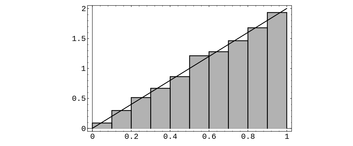
Running the program for 1000 darts resulted in the bar graph of Figure.
Note that here the heights of the bars are not all equal, but grow
approximately linearly with [math]r[/math]. In fact, the linear function [math]y = 2r[/math] appears
to fit our bar graph quite well. This suggests that the probability that the
dart falls within a distance [math]a[/math] of the center should be given by the
area under the graph of the function [math]y = 2r[/math] between 0 and [math]a[/math]. This area
is [math]a^2[/math], which agrees with the probability we have assigned above to this
event.
Sample Space Coordinates
These examples suggest that for continuous experiments of this sort we should assign probabilities for the outcomes to fall in a given interval by means of the area under a suitable function.
More generally, we suppose that suitable coordinates can be introduced into the
sample space [math]\Omega[/math], so that we can regard [math]\Omega[/math] as a subset of
[math]''' R'''^n[/math]. We call such a sample space a continuous sample space. We let
[math]X[/math] be a random variable which represents the outcome of the experiment. Such a
random variable is called a continuous random variable. We then define a density function for [math]X[/math] as follows.
Density Functions of Continuous Random Variables
Let [math]X[/math] be a continuous real-valued random variable. A density function for [math]X[/math] is a real-valued function [math]f[/math] which satisfies
We note that it is not the case that all continuous real-valued random variables possess density functions. However, in this book, we will only consider continuous random variables for which density functions exist.
In terms of the density [math]f(x)[/math], if [math]E[/math] is a subset of
[math]{\mat R}[/math], then
The notation here assumes that [math]E[/math] is a subset of [math]{\mat R}[/math] for which [math]\int_E f(x)\,dx[/math] makes sense.
Example In the spinner experiment, we choose for our set of outcomes the interval [math]0 \leq x \lt 1[/math], and for our density functionExample In the first dart game experiment, we choose for our sample space a disc of unit radius in the plane and for our density function the function
In these two examples, the density function is constant and does
not depend on the particular outcome. It is often the case that experiments in which the
coordinates are chosen at random can be described by constant
density functions, and, as in Section \ref{sec 1.2},
we call such density functions uniform or equiprobable. Not all experiments are of this type, however.
Example In the second dart game experiment, we choose for our sample space the unit interval on the real line and for our density the function
We see in this example that, unlike the case of discrete sample spaces, the
value [math]f(x)[/math] of the density function for the outcome [math]x[/math]
is not the probability of [math]x[/math] occurring (we have seen that this
probability is always 0) and in general [math]f(x)[/math] is not a probability
at all. In this example, if we take [math]\lambda = 2[/math] then [math]f(3/4) = 3/2[/math],
which being bigger than 1, cannot be a probability.
Nevertheless, the density function [math]f[/math] does contain all the
probability information about the experiment, since the probabilities of all
events can be derived from it. In particular, the probability that the outcome
of the experiment falls in an interval [math][a,b][/math] is given by
In the language of the calculus, we can say that the probability of occurrence
of an event of the form [math][x, x + dx][/math], where [math]dx[/math] is small,
is approximately given by
A glance at the graph of a density function tells us immediately
which events of an experiment are more likely. Roughly speaking, we can say
that where the density is large the events are more likely, and where it is
small the events are less likely. In Example the density function
is largest at 1. Thus, given the two intervals [math][0, a][/math] and [math][1, 1+a][/math], where [math]a[/math] is
a small positive real number, we see that [math]X[/math] is more likely to take on a value in the
second interval than in the first.
Cumulative Distribution Functions of Continuous Random Variables
We have seen that density functions are useful when considering continuous random variables. There is another kind of function, closely related to these density functions, which is also of great importance. These functions are called cumulative distribution functions.
Let [math]X[/math] be a continuous real-valued random variable. Then the cumulative distribution function of [math]X[/math] is defined by the equation
If [math]X[/math] is a continuous real-valued random variable which possesses a density function, then it also has a cumulative distribution function, and the following theorem shows that the two functions are related in a very nice way.
Let [math]X[/math] be a continuous real-valued random variable with density function [math]f(x)[/math]. Then the function defined by
By definition,
Applying the Fundamental Theorem of Calculus to the first equation in the statement of the theorem yields the second statement.
In many experiments, the density function of the relevant random variable is easy to
write down. However, it is quite often the case that the cumulative distribution function
is easier to obtain than the density function. (Of course, once we have the cumulative
distribution function, the density function can easily be obtained by differentiation, as
the above theorem shows.) We now give some examples which exhibit this phenomenon.
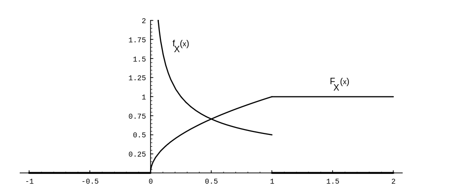
Example A real number is chosen at random from [math][0, 1][/math] with uniform probability, and then this number is squared. Let [math]X[/math] represent the result. What is the cumulative distribution function of [math]X[/math]? What is the density of [math]X[/math]?
We begin by letting [math]U[/math] represent the chosen real number. Then [math]X = U^2[/math]. If [math]0 \le x
\le 1[/math], then we have
When referring to a continuous random variable [math]X[/math] (say with a uniform density function), it is customary to say that “[math]X[/math] is uniformly distributed on the interval [math][a, b][/math].” It is also customary to refer to the cumulative distribution function of [math]X[/math] as the distribution function of [math]X[/math]. Thus, the word “distribution” is being used in several different ways in the subject of probability. (Recall that it also has a meaning when discussing discrete random variables.) When referring to the cumulative distribution function of a continuous random variable [math]X[/math], we will always use the word “cumulative” as a modifier, unless the use of another modifier, such as “normal” or “exponential,” makes it clear. Since the phrase “uniformly densitied on the interval [math][a, b][/math]” is not acceptable English, we will have to say “uniformly distributed” instead.
Example In Example, we considered a random variable, defined to be the sum of two random real numbers chosen uniformly from [math][0, 1][/math]. Let the random variables [math]X[/math] and [math]Y[/math] denote the two chosen real numbers. Define [math]Z = X + Y[/math]. We will now derive expressions for the cumulative distribution function and the density function of
[math]Z[/math].
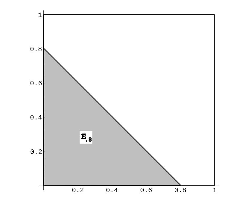

Here we take for our sample space [math]\Omega[/math] the unit square in [math]\mat{R}^2[/math]
with uniform density. A point [math]\omega \in \Omega[/math] then consists of a pair [math](x, y)[/math]
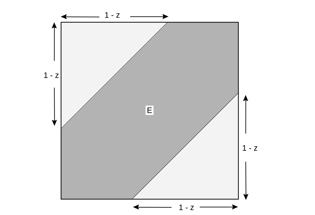
of numbers chosen at random. Then [math]0 \leq Z\leq 2[/math]. Let [math]E_z[/math] denote the event
that [math]Z \le z[/math]. In Figure, we show the set [math]E_{.8}[/math]. The event [math]E_z[/math],
for any [math]z[/math] between 0 and 1, looks very similar to the shaded set in the figure. For [math]1 \lt z
\le 2[/math], the set [math]E_z[/math] looks like the unit square with a triangle removed from the upper
right-hand corner. We can now calculate the probability distribution [math]F_Z[/math] of [math]Z[/math]; it is
given by
Example In the dart game described in Example, what is the distribution of the distance of the dart from the center of the target? What is its density?
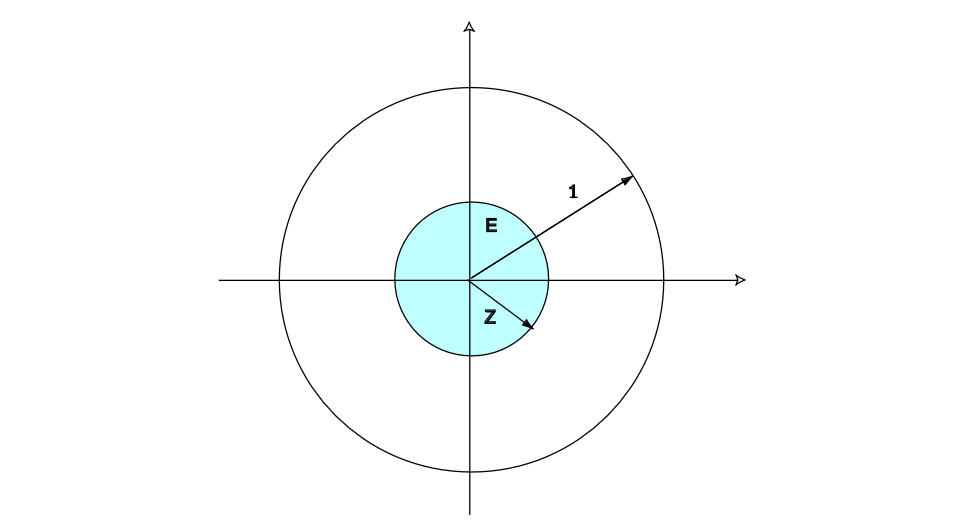
Here, as before, our sample space [math]\Omega[/math] is the unit disk in [math]\mat{R}^2[/math], with coordinates [math](X, Y)[/math]. Let [math]Z = \sqrt{X^2 + Y^2}[/math] represent the distance from the center of the target. Let [math]E[/math] be the event [math]\{Z \le z\}[/math]. Then the distribution function [math]F_Z[/math] of [math]Z[/math] (see Figure) is given by
We can verify this result by simulation, as follows: We choose values for [math]X[/math]
and [math]Y[/math] at random from [math][0,1][/math] with uniform distribution, calculate [math]Z =
\sqrt{X^2 + Y^2}[/math], check whether [math]0 \leq Z \leq 1[/math], and present the results in a
bar graph (see Figure).
Example Suppose Mr.\ and Mrs.\ Lockhorn agree to meet at the Hanover Inn between 5:00 and 6:00 {\scriptsize P.M.} on Tuesday. Suppose each arrives at a time between 5:00 and 6:00 chosen at random with uniform probability. What is the distribution function for the length of time that the first to arrive has to wait for the other? What is the density function?
Here again we can take the unit square to represent the sample space, and [math](X, Y)[/math]
as the arrival times (after 5:00 {\scriptsize P.M.}) for the Lockhorns. Let
[math]Z = |X - Y|[/math]. Then we have
[math]F_X(x) = x[/math] and [math]F_Y(y) = y[/math]. Moreover (see Figure),
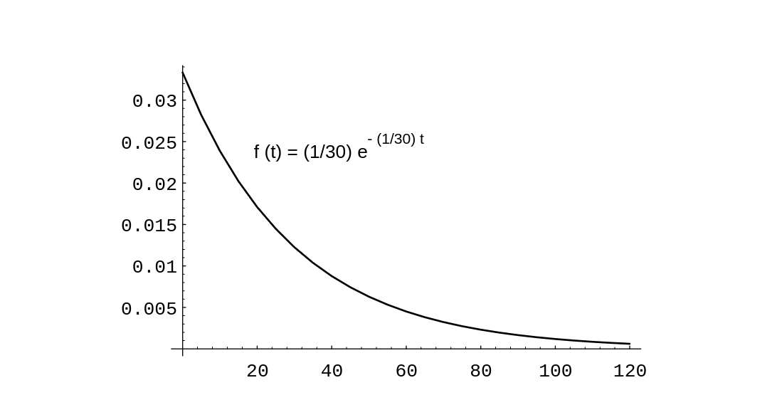
Example There are many occasions where we observe a sequence of occurrences which occur at “random” times. For example, we might be observing emissions of a radioactive isotope, or cars passing a milepost on a highway, or light bulbs burning out. In such cases, we might define a random variable [math]X[/math] to denote the time between successive occurrences. Clearly, [math]X[/math] is a continuous random variable whose range consists of the non-negative real numbers. It is often the case that we can model [math]X[/math] by using the exponential density. This density is given by the formula
One can see from the figure that even though the average value is 30, occasionally much larger values are taken on by [math]X[/math].
Suppose that we have bought a computer that contains a Warp 9 hard drive. The salesperson says that the average time between breakdowns of this type of hard
drive is 30 months. It is often assumed that the length of time between breakdowns is
distributed according to the exponential density. We will assume that this model applies
here, with
[math]\lambda = 1/30[/math].
Now suppose that we have been operating our computer for 15 months. We assume that the
original hard drive is still running. We ask how long we should expect the hard drive to
continue to run. One could reasonably expect that the hard drive will run, on the
average, another 15 months. (One might also guess that it will run more than 15 months,
since the fact that it has already run for 15 months implies that we don't have a lemon.)
The time which we have to wait is a new random variable, which we will call
[math]Y[/math]. Obviously, [math]Y = X - 15[/math]. We can write a computer program to produce a sequence of
simulated [math]Y[/math]-values. To do this, we first produce a sequence of [math]X[/math]'s, and discard those
values which are less than or equal to 15 (these values correspond to the cases where the
hard drive has quit running before 15 months). To simulate a value of
[math]X[/math], we compute the value of the expression
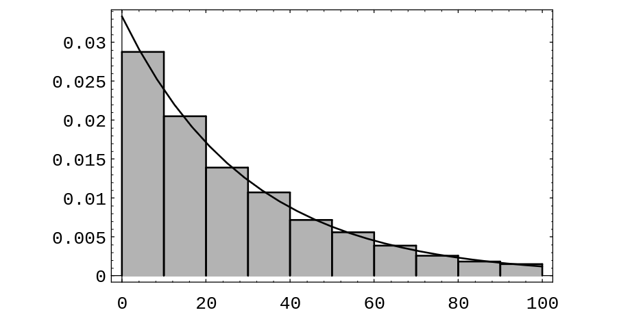
The average value of [math]Y[/math] in this simulation is 29.74, which is closer to the original
average life span of 30 months than to the value of 15 months which was guessed above.
Also, the distribution of [math]Y[/math] is seen to be close to the distribution of [math]X[/math]. It is in
fact the case that
[math]X[/math] and [math]Y[/math] have the same distribution. This property is called the memoryless
property, because the amount of time that we have to wait for an
occurrence does not depend on how long we have already waited. The only continuous density
function with this property is the exponential density.
Assignment of Probabilities
A fundamental question in practice is: How shall we choose the probability density function in describing any given experiment? The answer depends to a great extent on the amount and kind of information available to us about the experiment. In some cases, we can see that the outcomes are equally likely. In some cases, we can see that the experiment resembles another already described by a known density. In some cases, we can run the experiment a large number of times and make a reasonable guess at the density on the basis of the observed distribution of outcomes, as we did in Chapter Discrete Probability Distributions. In general, the problem of choosing the right density function for a given experiment is a central problem for the experimenter and is not always easy to solve (see Example). We shall not examine this question in detail here but instead shall assume that the right density is already known for each of the experiments under study. The introduction of suitable coordinates to describe a continuous sample space, and a suitable density to describe its probabilities, is not always so obvious, as our final example shows.
Infinite Tree
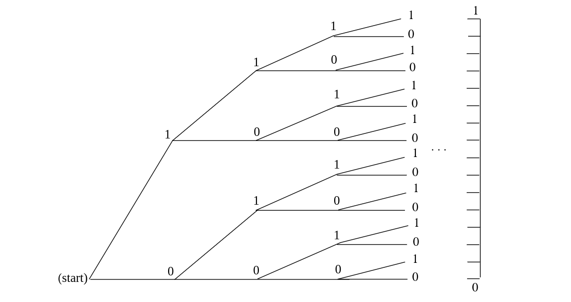
Example Consider an experiment in which a fair coin is tossed repeatedly, without stopping. We have seen in Example that, for a coin tossed [math]n[/math] times, the natural sample space is a binary tree with [math]n[/math] stages. On this evidence we expect that for a coin tossed repeatedly, the natural sample space is a binary tree with an infinite number of stages, as indicated in Figure. It is surprising to learn that, although the [math]n[/math]-stage tree is obviously a finite sample space, the unlimited tree can be described as a continuous sample space. To see how this comes about, let us agree that a typical outcome of the unlimited coin tossing experiment can be described by a sequence of the form [math]\omega = \{\mbox{H H T H T T H}\dots\}[/math]. If we write 1 for H and 0 for T, then [math]\omega = \{1\ 1\ 0\ 1\ 0\ 0\ 1\dots\}[/math]. In this way, each outcome is described by a sequence of 0's and 1's.
Now suppose we think of this sequence of 0's and 1's as the binary expansion of
some real number [math]x = .1101001\cdots[/math] lying between 0 and 1. (A binary expansion is like a decimal expansion but based on 2 instead of 10.)
Then each outcome is described by a value of [math]x[/math], and in this way [math]x[/math] becomes a
coordinate for the sample space, taking on all real values between 0 and 1. (We note that
it is possible for two different sequences to correspond to the same real number; for example,
the sequences [math]\{\mbox{T H H H H H}\ldots\}[/math] and [math]\{\mbox{H T T T T T}\ldots\}[/math] both
correspond to the real number [math]1/2[/math]. We will not concern ourselves with this apparent problem
here.)
What probabilities should be assigned to the events of this sample space?
Consider, for example, the event [math]E[/math] consisting of all outcomes for which the
first toss comes up heads and the second tails. Every such outcome has the
form [math].10****\cdots[/math], where [math]*[/math] can be either 0 or 1. Now if [math]x[/math] is our
real-valued coordinate, then the value of [math]x[/math] for every such outcome must lie
between [math]1/2 = .10000\cdots[/math] and [math]3/4 = .11000\cdots[/math], and moreover, every
value of [math]x[/math] between 1/2 and 3/4 has a binary expansion of the form
[math].10****\cdots[/math]. This means that [math]\omega\in E[/math] if and only if [math]1/2 \leq x \lt
3/4[/math], and in this way we see that we can describe [math]E[/math] by the interval
[math][1/2,3/4)[/math]. More generally, every event consisting of outcomes for which the
results of the first [math]n[/math] tosses are prescribed is described by a binary
interval of the form [math][k/2^n,(k+1)/2^n)[/math].
We have already seen in Section that in the experiment involving [math]n[/math] tosses, the probability of any one outcome must be exactly [math]1/2^n[/math]. It follows that in the unlimited toss experiment, the probability of any event consisting of outcomes for which the results of the first [math]n[/math] tosses are prescribed must also be [math]1/2^n[/math]. But [math]1/2^n[/math] is exactly the length of the interval of [math]x[/math]-values describing [math]E[/math]! Thus we see that, just as with the spinner experiment, the probability of an event [math]E[/math] is determined by what fraction of the unit interval lies in [math]E[/math]. Consider again the statement: The probability is 1/2 that a fair coin will turn up heads when tossed. We have suggested that one interpretation of this statement is that if we toss the coin indefinitely the proportion of heads will approach 1/2. That is, in our correspondence with binary sequences we expect to get a binary sequence with the proportion of 1's tending to 1/2. The event [math]E[/math] of binary sequences for which this is true is a proper subset of the set of all possible binary sequences. It does not contain, for example, the sequence [math]011011011\ldots[/math] (i.e., (011) repeated again and again). The event [math]E[/math] is actually a very complicated subset of the binary sequences, but its probability can be determined as a limit of probabilities for events with a finite number of outcomes whose probabilities are given by finite tree measures. When the probability of [math]E[/math] is computed in this way, its value is found to be 1. This remarkable result is known as the Strong Law of Large Numbers (or Law of Averages) and is one justification for our frequency concept of probability. We shall prove a weak form of this theorem in Chapter Law of Large Numbers.
General references
Doyle, Peter G. (2006). "Grinstead and Snell's Introduction to Probability" (PDF). Retrieved June 6, 2024.


