Penalty parameter selection, simulation, and illustration
[math] \require{textmacros} \def \bbeta {\bf \beta} \def\fat#1{\mbox{\boldmath$#1$}} \def\reminder#1{\marginpar{\rule[0pt]{1mm}{11pt}}\textbf{#1}} \def\SSigma{\bf \Sigma} \def\ttheta{\bf \theta} \def\aalpha{\bf \alpha} \def\bbeta{\bf \beta} \def\ddelta{\bf \delta} \def\eeta{\bf \eta} \def\llambda{\bf \lambda} \def\ggamma{\bf \gamma} \def\nnu{\bf \nu} \def\vvarepsilon{\bf \varepsilon} \def\mmu{\bf \mu} \def\nnu{\bf \nu} \def\ttau{\bf \tau} \def\SSigma{\bf \Sigma} \def\TTheta{\bf \Theta} \def\XXi{\bf \Xi} \def\PPi{\bf \Pi} \def\GGamma{\bf \Gamma} \def\DDelta{\bf \Delta} \def\ssigma{\bf \sigma} \def\UUpsilon{\bf \Upsilon} \def\PPsi{\bf \Psi} \def\PPhi{\bf \Phi} \def\LLambda{\bf \Lambda} \def\OOmega{\bf \Omega} [/math]
Penalty parameter selection
Throughout the introduction of the ridge regression estimator and the subsequent discussion of its properties, we considered the penalty parameter known or ‘given’. In practice, it is unknown and the user needs to make an informed decision on its value. We present several strategies to facilitate such a decision. Prior to that, we discuss some sanity requirements one may wish to impose on the ridge regression estimator. Those requirements do not yield a specific choice of the penalty parameter but they specify a domain of sensible penalty parameter values.
The evaluation of the ridge regression estimator may be subject to numerical inaccuracy, which ideally is avoided. This numerical inaccuracy results from the ill-conditionedness of [math]\mathbf{X}^{\top} \mathbf{X} + \lambda \mathbf{I}_{pp}[/math]. A matrix is ill-conditioned if its condition number is high. The condition number of a square positive definite matrix [math]\mathbf{A}[/math] is the ratio of its largest and smallest eigenvalue. If the smallest eigenvalue is zero, the conditional number is undefined and so is [math]\mathbf{A}^{-1}[/math]. Furthermore, a high condition number is indicative of the loss (on a log-scale) in numerical accuracy of the evaluation of [math]\mathbf{A}^{-1}[/math]. To ensure the numerical accurate evaluation of the ridge regression estimator, the choice of the penalty parameter is thus to be restricted to a subset of the positive real numbers such that it yields a well-conditioned matrix [math]\mathbf{X}^{\top} \mathbf{X} + \lambda \mathbf{I}_{pp}[/math]. Clearly, the penalty parameter [math]\lambda[/math] should then not be too close to zero. There is however no consensus on the criteria on the condition number for a matrix to be well-defined. This depends among others on how much numerical inaccuracy is tolerated by the context. Of course, as pointed out in Section Computationally efficient evaluation , inversion of the [math]\mathbf{X}^{\top} \mathbf{X} + \lambda \mathbf{I}_{pp}[/math] matrix can be circumvented. One then still needs to ensure the well-conditionedness of [math]\lambda^{-1} \mathbf{X} \mathbf{X}^{\top} + \mathbf{I}_{nn}[/math], which too results in a lower bound for the penalty parameter. Practically, following [1] (who do so in a different context), we suggest to generate a conditional number plot. It plots (on some convenient scale) the condition number of the matrix [math]\mathbf{X}^{\top} \mathbf{X} + \lambda \mathbf{I}_{pp}[/math] against the penalty parameter [math]\lambda[/math]. From this plot, we identify the domain of the penalty parameter value associated with well-conditionedness. To guide in this choice, [1] overlay this plot with a curve indicative of the numerical inaccurary.
Traditional text books on regression analysis suggest, in order to prevent over-fitting, to limit the number of covariates of the model. In addition, this ought to leave enough degrees of freedom to estimate the error and facilitate proper inference. While ridge regression is commonly used for prediction purposes and inference need not be the objective, over-fitting is certainly to be avoided. This can be achieved by limiting the degrees of freedom spent on the estimation of the regression parameter. We thus follow [2] and use the degrees of freedom to bound the search domain of the penalty parameter. This requires the specification of a maximum degrees of freedom one wishes to spend on the construction of the ridge regression estimator. Denote this by [math]\nu[/math], and recall that [math]0\leq \nu \leq n[/math]. Then, choose [math]\lambda[/math] such that [math]\mbox{tr}[ \mathbf{H}(\lambda)] \leq \nu[/math]. To find the bound on the penalty parameter, note that
Then, if [math]\lambda \geq \max\{ 0, \nu^{-1} [d_1 (\mathbf{X})]^2 (p - \nu)\}[/math], the degrees of freedom consumed by the ridge regression estmator is smaller than [math]\nu[/math].
Information criterion
A popular strategy is to choose a penalty parameter that yields a good but parsimonious model. Information criteria measure the balance between model fit and model complexity. Here we present the Aikaike's information criterion (AIC), but many other criteria have been presented in the literature (e.g. [3], [4]). The AIC measures model fit by the loglikelihood and model complexity as measured by the number of parameters used by the model. The number of model parameters in regular regression simply corresponds to the number of covariates in the model. Or, by the degrees of freedom consumed by the model, which is equivalent to the trace of the hat matrix. For ridge regression it thus seems natural to define model complexity analogously by the trace of the ridge hat matrix. This yields the AIC for the linear regression model with ridge regression estimates:
as [math]\hat{\sigma}^{-2}(\lambda) = n^{-1} \| \mathbf{Y} - \mathbf{X} \hat{\bbeta}(\lambda) \|_2^2[/math]. The value of [math]\lambda[/math] which minimizes [math]\mbox{AIC}(\lambda)[/math] corresponds to the ‘optimal’ balance of model complexity and overfitting.
Information criteria guide the decision process when having to decide among various different models. Different models use different sets of explanatory variables to explain the behaviour of the response variable. In that sense, the use of information criteria for the deciding on the ridge penalty parameter may be considered inappropriate: ridge regression uses the same set of explanatory variables irrespective of the value of the penalty parameter. Moreover, often ridge regression is employed to predict a response and not to provide an insightful explanatory model. The latter need not yield the best predictions. Finally, empirically we observe that the AIC often does not show an optimum inside but at the boundaries of the domain of the ridge penalty parameter. Henceforth, we refrain from the use of the AIC (or any of its relatives) in determining the optimal ridge penalty parameter.
Cross-validation
Instead of choosing the penalty parameter to balance model fit with model complexity, cross-validation requires it (i.e. the penalty parameter) to yield a model with good prediction performance. Commonly, this performance is evaluated on novel data. Novel data need not be easy to come by and one has to make do with the data at hand. The setting of ‘original’ and novel data is then mimicked by sample splitting: the data set is divided into two (groups of samples). One of these two data sets, called the training set, plays the role of ‘original’ data on which the model is built. The second of these data sets, called the test set, plays the role of the ‘novel’ data and is used to evaluate the prediction performance (often operationalized as the loglikelihood or the prediction error) of the model built on the training data set. This procedure (model building and prediction evaluation on training and test set, respectively) is done for a collection of possible penalty parameter choices. The penalty parameter that yields the model with the best prediction performance is to be preferred. The thus obtained performance evaluation depends on the actual split of the data set. To remove this dependence, the data set is split many times into a training and test set. Per split the model parameters are estimated for all choices of [math]\lambda[/math] using the training data and estimated parameters are evaluated on the corresponding test set. The penalty parameter, that on average over the test sets performs best (in some sense), is then selected.
When the repetitive splitting of the data set is done randomly, samples may accidently end up in a fast majority of the splits in either training or test set. Such samples may have an unbalanced influence on either model building or prediction evaluation. To avoid this [math]k[/math]-fold cross-validation structures the data splitting. The samples are divided into [math]k[/math] more or less equally sized exhaustive and mutually exclusive subsets. In turn (at each split) one of these subsets plays the role of the test set while the union of the remaining subsets constitutes the training set. Such a splitting warrants a balanced representation of each sample in both training and test set over the splits. Still the division into the [math]k[/math] subsets involves a degree of randomness. This may be fully excluded when choosing [math]k=n[/math]. This particular case is referred to as leave-one-out cross-validation (LOOCV). For illustration purposes the LOOCV procedure is detailed fully below:
- Define a range of interest for the penalty parameter.
- Divide the data set into training and test set comprising samples [math]\{1, \ldots, n\} \setminus i[/math] and [math]\{ i \}[/math], respectively.
- Fit the linear regression model by means of ridge estimation for each [math]\lambda[/math] in the grid using the training set. This yields:
[[math]] \begin{eqnarray*} \hat{\bbeta}_{-i}(\lambda) & = & ( \mathbf{X}_{-i, \ast}^{\top} \mathbf{X}_{-i, \ast} + \lambda \mathbf{I}_{pp})^{-1} \mathbf{X}_{-i, \ast}^{\top} \mathbf{Y}_{-i} \end{eqnarray*} [[/math]]and the corresponding estimate of the error variance [math]\hat{\sigma}_{-i}^2(\lambda)[/math].
- Evaluate the prediction performance of these models on the test set by [math]\log\{L[Y_i, \mathbf{X}_{i, \ast}; \hat{\bbeta}_{-i}(\lambda), \hat{\sigma}_{-i}^2(\lambda)]\}[/math]. Or, by the prediction error [math]|Y_i - \mathbf{X}_{i, \ast} \hat{\bbeta}_{-i}(\lambda)|[/math], possibly squared.
- Repeat steps 1) to 3) such that each sample plays the role of the test set once.
- Average the prediction performances of the test sets at each grid point of the penalty parameter:
[[math]] \begin{eqnarray*} n^{-1} \sum\nolimits_{i = 1}^n \log\{L[Y_i, \mathbf{X}_{i, \ast}; \hat{\bbeta}_{-i}(\lambda), \hat{\sigma}_{-i}^2(\lambda)]\}. \end{eqnarray*} [[/math]]The quantity above is called the cross-validated loglikelihood. It is an estimate of the prediction performance of the model corresponding to this value of the penalty parameter on novel data.
- The value of the penalty parameter that maximizes the cross-validated loglikelihood is the value of choice.
The procedure is straightforwardly adopted to [math]k[/math]-fold cross-validation, a different criterion, and different estimators.
In the LOOCV procedure above resampling can be avoided when the predictive performance is measured by Allen's PRESS (Predicted Residual Error Sum of Squares) statistic [5]. For then, the LOOCV predictive performance can be expressed analytically in terms of the known quantities derived from the design matrix and response (as pointed out but not detailed in [6]). Define the optimal penalty parameter to minimize Allen's PRESS statistic:
where [math]\mathbf{B}(\lambda)[/math] is diagonal with [math][\mathbf{B}(\lambda)]_{ii} = [ 1 - \mathbf{H}_{ii}(\lambda)]^{-1}[/math]. The second equality in the preceding display is elaborated in Exercise. Its main takeaway is that the predictive performance for a given [math]\lambda[/math] can be assessed directly from the ridge hat matrix and the response vector without the recalculation of the [math]n[/math] leave-one-out ridge regression estimators. Computationally, this is a considerable gain.
No such analytic expression of the cross-validated loss as above exists for general [math]K[/math]-fold cross-validation, but considerable computational gain can nonetheless be achieved [7]. This exploits the fact that the ridge regression estimator appears in Allen's PRESS statistics -- and the likelihood -- only in combination with the design matrix, together forming the linear predictor. There is thus no need to evaluate the estimator itself when interest is only in its predictive performance. Then, if [math]\mathcal{G}_1, \ldots, \mathcal{G}_K \subset \{1, \ldots, n\}[/math] are the mutually exclusive and exhaustive [math]K[/math]-fold sample index sets, the linear predictor for the [math]k[/math]-th fold can be expressed as:
where we have used the Woodbury identity again. Finally, for each fold the computationally most demanding matrices of this expression, [math]\mathbf{X}_{\mathcal{G}_k, \ast} \mathbf{X}_{-\mathcal{G}_k, \ast}^{\top}[/math] and [math]\mathbf{X}_{-\mathcal{G}_k, \ast} \mathbf{X}_{-\mathcal{G}_k, \ast}^{\top}[/math], are both submatrices of [math]\mathbf{X} \mathbf{X}^{\top}[/math]. If this matrix is evaluated prior to the cross-validation loop, all calculations inside the loop involve only matrices of dimensions [math]n \times n[/math], maximally.
Generalized cross-validation
Generalized cross-validation is another method to guide the choice of the penalty parameter. It is like cross-validation but with a different criterion to evaluate the performance of the ridge regression estimator on novel data. This criterion, denoted [math]\mbox{GCV}(\lambda)[/math] (where GCV is an acronym of Generalized Cross-Validation), is an approximation to Allen's PRESS statistic. In the previous subsection this statistic was reformulated as:
The identity [math]\mbox{tr}[\mathbf{H}(\lambda)] = \sum_{i=1}^n [\mathbf{H}(\lambda)]_{ii}[/math] suggests [math][\mathbf{H}(\lambda)]_{ii} \approx n^{-1} \mbox{tr}[\mathbf{H}(\lambda)][/math]. The approximation thus proposed by [6], which they endow with a ‘weighted version of Allen’s PRESS statistic'-interpretation, is:
The need for this approximation is pointed out by [6] by example through an ‘extreme’ case where the minimization of Allen's PRESS statistic fails to produce a well-defined choice of the penalty parameter [math]\lambda[/math]. This ‘extreme’ case requires a (unit) diagonal design matrix [math]\mathbf{X}[/math]. Straightforward (linear) algebraic manipulations of Allen's PRESS statistic then yield:
which indeed has no unique minimizer in [math]\lambda[/math]. Additionally, the [math]\mbox{GCV}(\lambda)[/math] criterion may in some cases be preferred computationally when it is easier to evaluate [math]\mbox{tr}[ \mathbf{H}(\lambda)][/math] (e.g. from the singular values) than the individual diagonal elements of [math]\mathbf{H}(\lambda)[/math]. Finally, [8] showed that the [math]\lambda[/math] that minimizes [math]\mbox{GCV}(\lambda)[/math] is optimal asymptotically (i.e. for ever larger sample sizes).
Randomness
The discussed procedures for penalty parameter selection all depend on the data at hand. As a result, so does the selected penalty parameter. It should therefore be considered a statistic, a quantity calculated from data. In case of [math]K[/math]-fold cross-validation, the random formation of the splits adds another layer of randomness. Irrespectively, a statistic exhibits randomness. This randomness that propagates into the ridge regression estimator. The distributional properties of the ridge regression estimator derived in Section Moments are thus conditional on the penalty parameter.
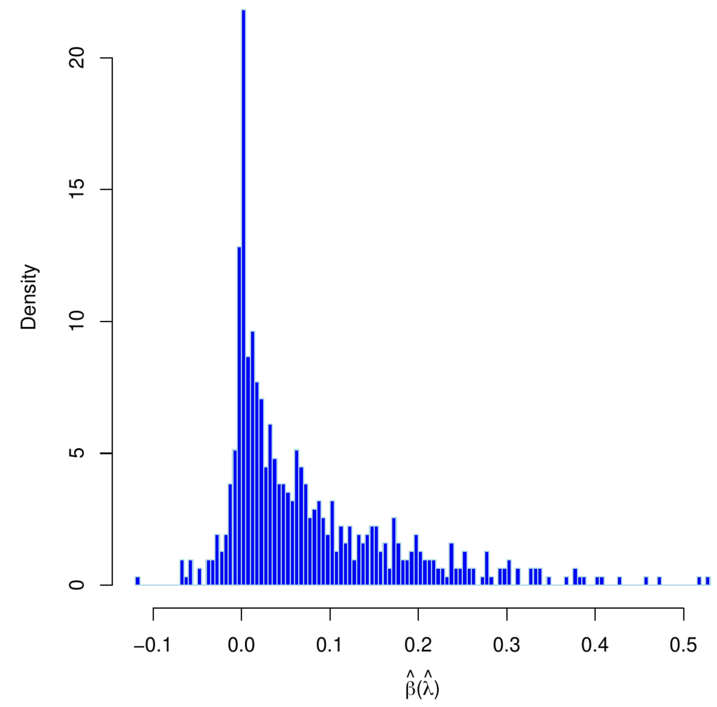
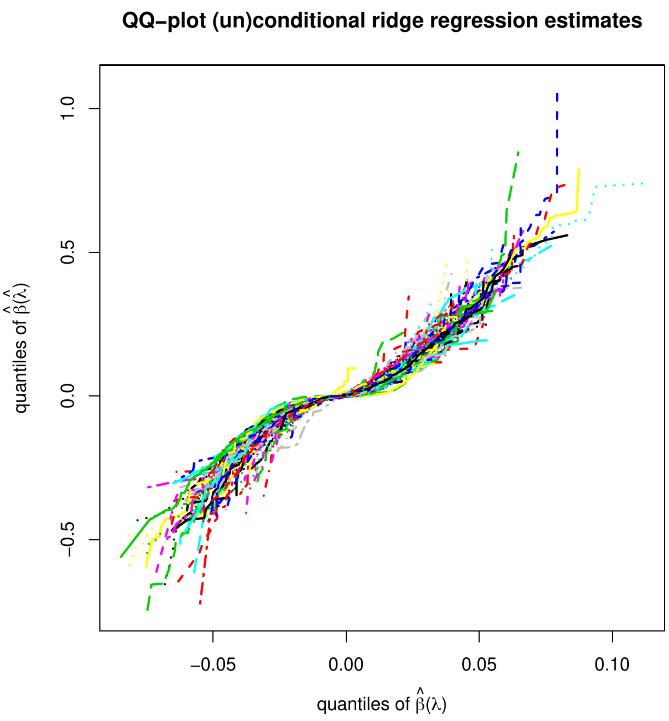
Left panel: histogram of estimates of an element of [math]\hat{\bbeta}(\hat{\lambda})[/math] obtained from thousand bootstrap samples with re-tuned penalty parameters. Right penal: qq-plot of the estimates estimates of an element of [math]\hat{\bbeta}(\hat{\lambda})[/math] obtained from thousand bootstrap samples with re-tuned vs. fixed penalty parameters.
Those of the unconditional distribution of the ridge regression estimator, now denoted [math]\hat{\bbeta}(\hat{\lambda})[/math] with [math]\hat{\lambda}[/math] indicating that the penalty depends on the data (and possibly the particulars of the splits), may be rather different. Analytic finite sample results appear to be unavailable. An impression of the distribution of [math]\hat{\bbeta}(\hat{\lambda})[/math] can be obtained through simulation. Hereto we have first drawn a data set from the linear regression model with dimension [math]p=100[/math], sample size [math]n=25[/math], a standard normally distribution error, the rows of the design matrix sampled from a zero-centered multivariate normal distribution with a uniformly correlated but equivariant covariance matrix, and a regression parameter with elements equidistantly distributed over the interval [math][-2\tfrac{1}{2}, 2 \tfrac{1}{2}][/math]. From this data set, we then generate thousand nonparametric bootstrapped data sets. For each bootstrapped data set, we select the penalty parameter by means of [math]K=10[/math]-fold cross-validation and evaluate the ridge regression estimator using the selected penalty parameter. The left panel of Figure shows the histogram of the thus acquired estimates of an arbitrary element of the regression parameter. The shape of the distribution clearly deviates from the normal one of the conditional ridge regression estimator. In the right panel of Figure, we have plotted element-wise quantiles of the conditional vs. unconditional ridge regression estimators. It reveals that not only the shape of the distribution, but also its moments are affected by the randomness of the penalty parameter.
Simulations
Simulations are presented that illustrate properties of the ridge regression estimator not discussed explicitly in the previous sections of this chapter.
Role of the variance of the covariates
In many applications of high-dimensional data the covariates are standardized prior to the execution of the ridge regression. Before we discuss whether this is appropriate, we first illustrate the effect of ridge penalization on covariates with distinct variances using simulated data.
The simulation involves one response to be (ridge) regressed on fifty covariates. Data (with [math]n=1000[/math]) for the covariates, denoted [math]\mathbf{X}[/math], are drawn from a multivariate normal distribution: [math]\mathbf{X} \sim \mathcal{N}(\mathbf{0}_{50}, \mathbf{\Sigma})[/math] with [math]\mathbf{\Sigma}[/math] diagonal and [math](\mathbf{\Sigma})_{jj} = j / 10[/math]. From this the response is generated through [math]\mathbf{Y} = \mathbf{X} \bbeta + \vvarepsilon[/math] with [math]\bbeta = \mathbf{1}_{50}[/math] and [math]\vvarepsilon \sim \mathcal{N}(\mathbf{0}_{50}, \mathbf{I}_{50 \times 50})[/math].
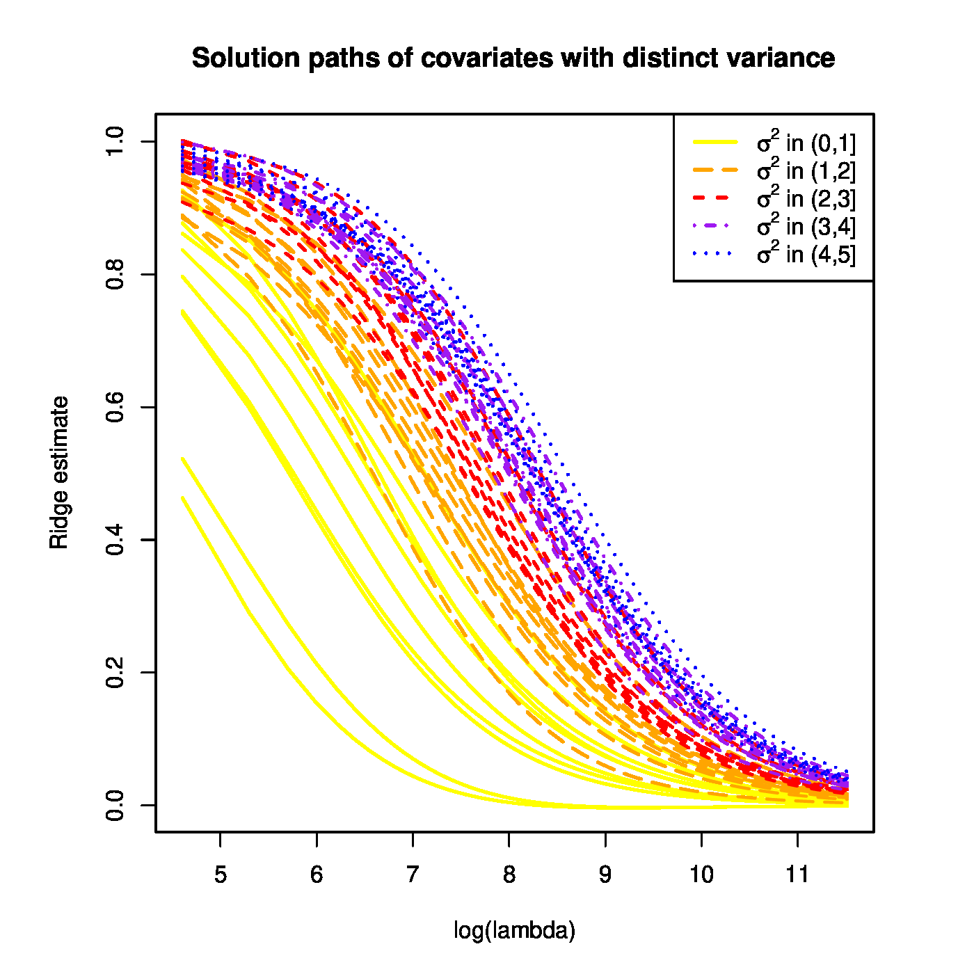
With the simulated data at hand the ridge regression estimates of [math]\bbeta[/math] are evaluated for a large grid of the penalty parameter [math]\lambda[/math]. The resulting ridge regularization paths of the regression coefficients are plotted (Figure). All paths start ([math]\lambda=0[/math]) close to one and vanish as [math]\lambda \rightarrow \infty[/math]. However, ridge regularization paths of regression coefficients corresponding to covariates with a large variance dominate those with a low variance.
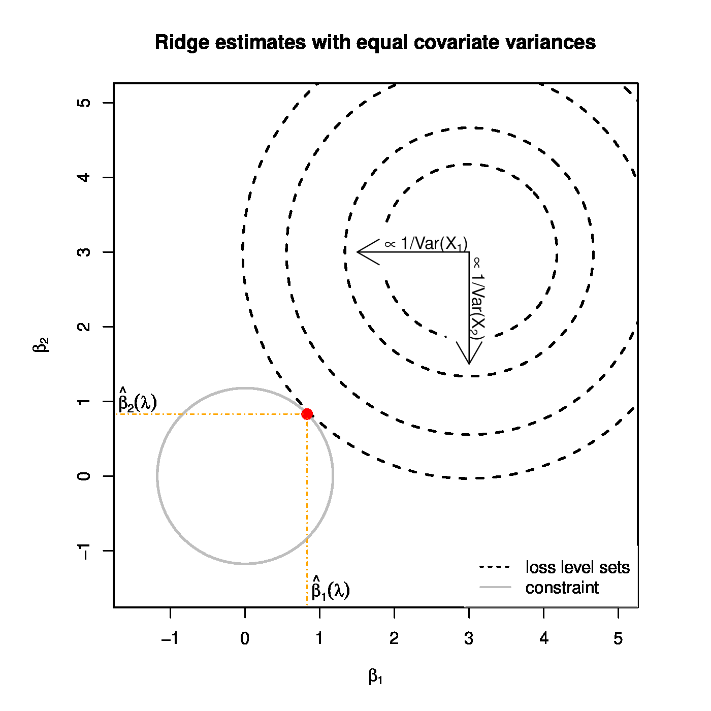
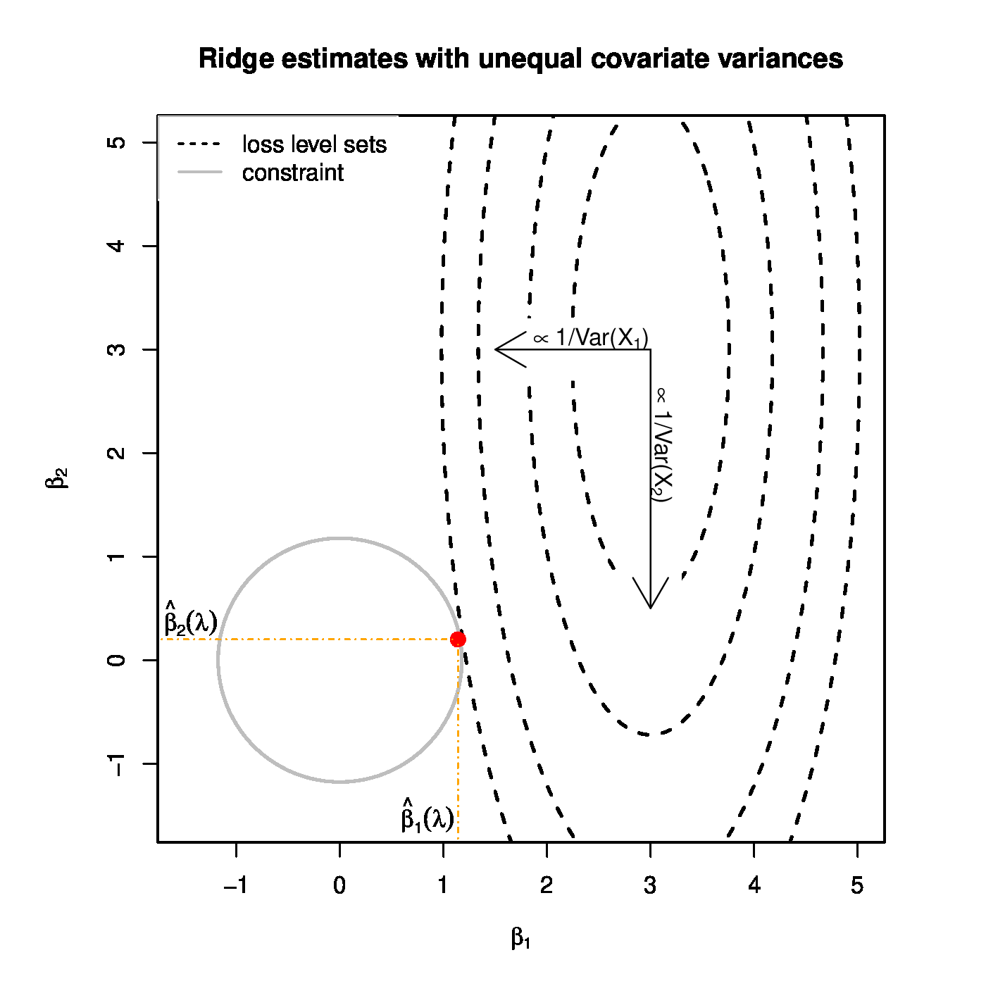
Top panel: Ridge regularization paths for coefficients of the 50 uncorrelated covariates with distinct variances. Color and line type indicated the grouping of the covariates by their variance. Bottom panels: Graphical illustration of the effect of a covariate's variance on the ridge estimator. The grey circle depicts the ridge parameter constraint. The dashed black ellipsoids are the level sets of the least squares loss function. The red dot is the ridge regression estimate. Left and right panels represent the cases with equal and unequal, respectively, variances of the covariates.
Ridge regression's preference of covariates with a large variance can intuitively be understood as follows. First note that the ridge regression estimator now can be written as:
Plug in the employed parametrization of [math]\mathbf{\Sigma}[/math], which gives: [math][\bbeta (\lambda)]_j = j (j + 50 \lambda)^{-1} (\bbeta)_j[/math]. Hence, the larger the covariate's variance (corresponding to the larger [math]j[/math]), the larger its ridge regression coefficient estimate. Ridge regression thus prefers, among a set of covariates with comparable effect sizes, those with larger variances.
The reformulation of ridge penalized estimation as a constrained estimation problem offers a geometrical interpretation of this phenomenon. Let [math]p=2[/math] and the design matrix [math]\mathbf{X}[/math] be orthogonal, while both covariates contribute equally to the response. Contrast the cases with [math]\mbox{Var}(X_1) \approx \mbox{Var}(X_2)[/math] and [math]\mbox{Var}(X_1) \gg \mbox{Var}(X_2)[/math]. The level sets of the least squares loss function associated with the former case are circular, while that of the latter are strongly ellipsoidal (see Figure). The diameters along the principal axes (that -- due to the orthogonality of [math]\mathbf{X}[/math] -- are parallel to that of the [math]\beta_1[/math]- and [math]\beta_2[/math]-axes) of both circle and ellipsoid are reciprocals of the variance of the covariates. When the variances of both covariates are equal, the level sets of the loss function expand equally fast along both axes. With the two covariates having the same regression coefficient, the point of these level sets closest to the parameter constraint is to be found on the line [math]\beta_1 = \beta_2[/math] (Figure, left panel). Consequently, the ridge regression estimator satisfies [math]\hat{\beta}_1 (\lambda) \approx \hat{\beta}_2(\lambda)[/math]. With unequal variances between the covariates, the ellipsoidal level sets of the loss function have diameters of rather different sizes. In particular, along the [math]\beta_1[/math]-axis it is narrow (as [math]\mbox{Var}(X_1)[/math] is large), and -- vice versa -- wide along the [math]\beta_2[/math]-axis. Consequently, the point of these level sets closest to the circular parameter constraint will be closer to the [math]\beta_1[/math]- than to the [math]\beta_2[/math]-axis (Figure, left panel). For the ridge estimator of the regression parameter this implies [math]0 \ll \hat{\beta}_1 (\lambda) \lt 1[/math] and [math]0 \lt \hat{\beta}_2 (\lambda) \ll 1[/math]. Hence, the covariate with a larger variance yields the larger ridge regression estimator.
Should one thus standardize the covariates prior to ridge regression analysis? When dealing with gene expression data from microarrays, the data have been subjected to a series of pre-processing steps (e.g. quality control, background correction, within- and between-normalization). The purpose of these steps is to make the expression levels of genes comparable both within and between hybridizations. The preprocessing should thus be considered an inherent part of the measurement. As such, it is to be done independently of whatever down-stream analysis is to follow and further tinkering with the data is preferably to be avoided (as it may mess up the ‘comparable-ness’ of the expression levels as achieved by the preprocessing). For other data types different considerations may apply.
Among the considerations to decide on standardization of the covariates, one should also include the fact that ridge regression estimates prior and posterior to scaling do not simply differ by a factor. To see this assume that the covariates have been centered. Scaling of the covariates amounts to post-multiplication of the design matrix by a [math]p \times p[/math]-dimensional diagonal matrix [math]\mathbf{A}[/math] with the reciprocals of the covariates' scale estimates on its diagonal [9]. Hence, the ridge regression estimator (for the rescaled data) is then given by:
Apply the change-of-variable [math]\ggamma = \mathbf{A} \bbeta[/math] and obtain:
Effectively, the scaling is equivalent to covariate-wise penalization (see Chapter Generalizing ridge regression for more on this). The ‘scaled’ ridge regression estimator may then be derived along the same lines as before in Section Constrained estimation :
In general, this is unequal to the ridge estimator without the rescaling of the columns of the design matrix. Moreover, it should be clear that [math]\hat{\bbeta}^{\mbox{{\tiny (scaled)}}} (\lambda) \not= \mathbf{A} \hat{\bbeta}(\lambda)[/math].
Ridge regression and collinearity
Initially, ridge regression was motivated as an ad-hoc fix of (super)-collinear covariates in order to obtain a well-defined estimator. We now study the effect of this ad-hoc fix on the regression coefficient estimates of collinear covariates. In particular, their ridge regularization paths are contrasted to those of ‘non-collinear’ covariates.
To this end, we consider a simulation in which one response is regressed on 50 covariates. The data of these covariates, stored in a design matrix denoted [math]\mathbf{X}[/math], are sampled from a multivariate normal distribution, with mean zero and a [math]5 \times 5[/math] block covariance matrix:
with
The data of the response variable [math]\mathbf{Y}[/math] are then obtained through: [math]\mathbf{Y} = \mathbf{X} \bbeta + \vvarepsilon[/math], with [math]\vvarepsilon \sim \mathcal{N}( \mathbf{0}_{n}, \mathbf{I}_{nn})[/math] and [math]\bbeta = \mathbf{1}_{50}[/math]. Hence, all covariates contribute equally to the response. Would the columns of [math]\mathbf{X}[/math] be orthogonal, little difference in the ridge estimates of the regression coefficients is expected.
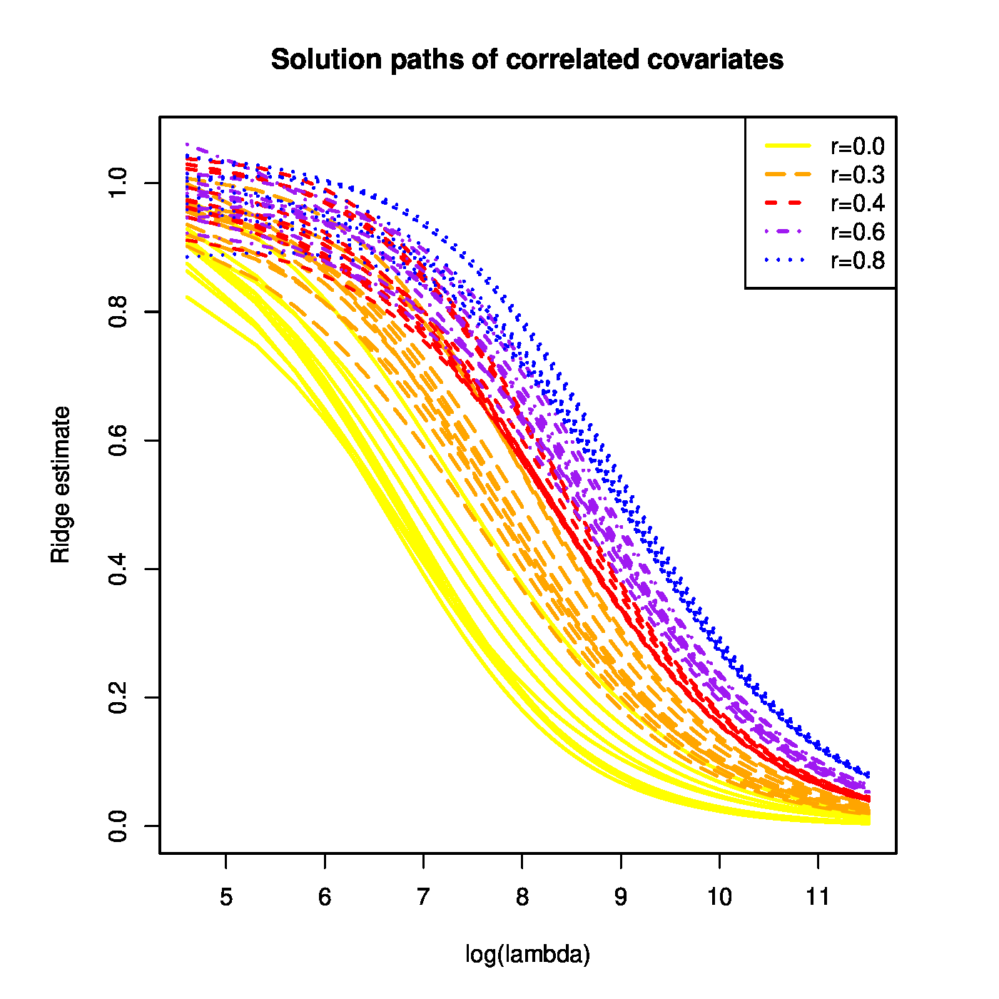
The results of this simulation study with sample size [math]n=1000[/math] are presented in Figure. All 50 regularization paths start close to one as [math]\lambda[/math] is small and converge to zero as [math]\lambda \rightarrow \infty[/math]. But the paths of covariates of the same block of the covariance matrix [math]\mathbf{\Sigma}[/math] quickly group, with those corresponding to a block with larger off-diagonal elements above those with smaller ones. Thus, ridge regression prefers (i.e. shrinks less) coefficient estimates of strongly positively correlated covariates.
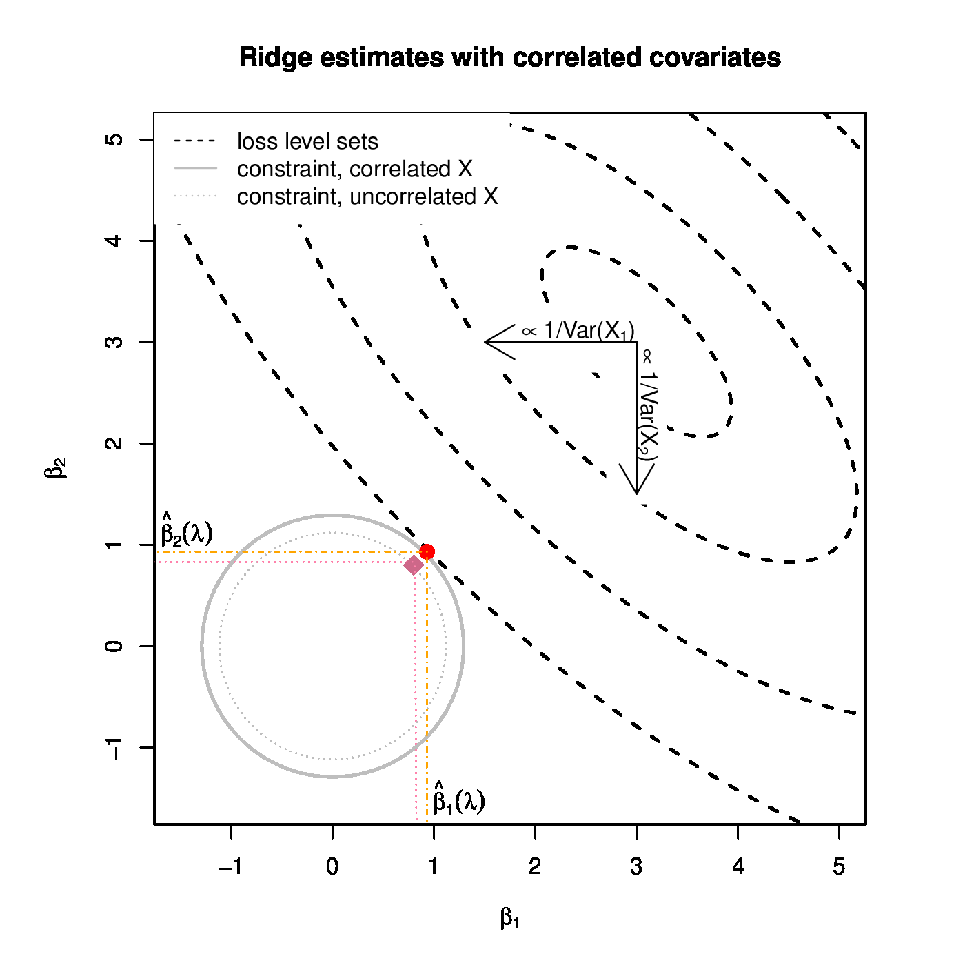
Left panel: Ridge regularization paths for coefficients of the 50 covariates, with various degree of collinearity but equal variance. Color and line type correspond to the five blocks of the covariate matrix [math]\mathbf{\Sigma}[/math]. Right panel: Graphical illustration of the effect of the collinearity among covariates on the ridge estimator. The solid and dotted grey circles depict the ridge parameter constraint for the collinear and orthogonal cases, respectively. The dashed black ellipsoids are the level sets of the sum-of-squares squares loss function. The red dot and violet diamond are the ridge regression for the positive collinear and orthogonal case, respectively.
Intuitive understanding of the observed behaviour may be obtained from the [math]p=2[/math] case. Let [math]U[/math], [math]V[/math] and [math]\varepsilon[/math] be independent random variables with zero mean. Define [math]X_1 = U + V[/math], [math]X_2 = U - V[/math], and [math]Y = \beta_1 X_1 + \beta_2 X_2 + \varepsilon[/math] with [math]\beta_1[/math] and [math]\beta_2[/math] constants. Hence, [math]\mathbb{E}(Y) = 0[/math]. Then:
and [math]\mbox{Cor}(X_{1}, X_{2}) = [\mbox{Var}(U) - \mbox{Var}(V)] / [ \mbox{Var}(U) + \mbox{Var}(V) ][/math]. The random variables [math]X_1[/math] and [math]X_2[/math] are strongly positively correlated if [math]\mbox{Var}(U) \gg \mbox{Var}(V)[/math]. The ridge regression estimator associated with regression of [math]Y[/math] on [math]U[/math] and [math]V[/math] is:
For large enough [math]\lambda[/math]
When [math]\mbox{Var}(U) \gg \mbox{Var}(V)[/math] and [math]\beta_1 \approx \beta_2[/math], the ridge estimate of [math]\gamma_v[/math] vanishes for large [math]\lambda[/math]. Hence, ridge regression prefers positively covariates with similar effect sizes.
This phenomenon can also be explained geometrically. For the illustration consider ridge estimation with [math]\lambda=1[/math] of the linear model [math]\mathbf{Y} = \mathbf{X} \bbeta + \vvarepsilon[/math] with [math]\bbeta = (3, 3)^{\top}[/math], [math]\vvarepsilon \sim \mathcal{N}(\mathbf{0}_2, \mathbf{I}_{22})[/math] and the columns of [math]\mathbf{X}[/math] strongly and positively collinear. The level sets of the sum-of-squares loss, [math]\| \mathbf{Y} - \mathbf{X} \bbeta \|_2^2[/math], are plotted in the right panel of Figure. Recall that the ridge regression estimate is found by looking for the smallest loss level set that hits the ridge contraint. The sought-for estimate is then the point of intersection between this level set and the constraint, and -- for the case at hand -- is on the [math]x=y[/math]-line. This is no different from the case with orthogonal [math]\mathbf{X}[/math] columns. Yet their estimates differ, even though the same [math]\lambda[/math] is applied. The difference is to due to fact that the radius of the ridge constraint depends on [math]\lambda[/math], [math]\mathbf{X}[/math] and [math]\mathbf{Y}[/math]. This is immediate from the fact that the radius of the constraint equals [math]\| \hat{\bbeta}(\lambda) \|_2^2[/math] (see Section Constrained estimation ). To study the effect of [math]\mathbf{X}[/math] on the radius, we remove its dependence on [math]\mathbf{Y}[/math] by considering its expectation, which is:
In the last step we have used [math]\mathbf{Y} \sim \mathcal{N}( \mathbf{X} \bbeta, \sigma^2 \mathbf{I}_{pp})[/math] and the expectation of the quadratic form of a multivariate random variable [math]\vvarepsilon \sim \mathcal{N}(\mmu_{\varepsilon}, \SSigma_{\varepsilon})[/math] is [math]\mathbb{E} ( \vvarepsilon^{\top} \LLambda \, \vvarepsilon) = \mbox{tr} ( \LLambda \, \SSigma_{\varepsilon}) + \mmu_{\varepsilon}^{\top} \LLambda \mmu_{\varepsilon}[/math] (cf. [10]). The expression for the expectation of the radius of the ridge constraint can now be evaluated for the orthogonal [math]\mathbf{X}[/math] and the strongly, positively collinear [math]\mathbf{X}[/math]. It turns out that the latter is larger than the former. This results in a larger ridge constraint. For the larger ridge constraint there is a smaller level set that hits it first. The point of intersection, still on the [math]x=y[/math]-line, is now thus closer to [math]\bbeta[/math] and further from the origin (cf. right panel of Figure). The resulting estimate is thus larger than that from the orthogonal case.
The above needs some attenuation. Among others it depends on:
- the number of covariates in each block,
- the size of the effects, i.e. regression coefficients of each covariate,
- and the degree of collinearity. Possibly, there are more factors influencing the behaviour of the ridge estimator presented in this subsection.
This behaviour of ridge regression is to be understood if a certain (say) clinical outcome is to be predicted from (say) gene expression data. Genes work in concert to fulfil a certain function in the cell. Consequently, one expects their expression levels to be correlated. Indeed, gene expression studies exhibit many co-expressed genes, that is, genes with correlating transcript levels. But also in most other applications with many explanatory variables collinearity will be omnipresent and similar issues are to be considered.
Variance inflation factor
The ridge regression estimator was introduced to resolve the undefinedness of its maximum likelihood counterpart in the face of (super)collinearity amoung the explanatory variables. The effect of collinearity on the uncertainty of estimates is often quantified by the Variance Inflation Factor (VIF). The VIF measures the change in the variance of the estimate due to the collinearity. Here we investigate how penalization affects the VIF. This requires a definition of the VIF of the ridge regression estimator.
The VIF of the maximum likelihood estimator of the [math]j[/math]-th element of the regression parameter is defined as a factor in the following factorization of the variance of [math]\hat{\beta}_j[/math]:
in which it assumed that the [math]X_{i,j}[/math]'s are random and -- using the column-wise zero ‘centered-ness’of [math]\mathbf{X}[/math] -- that [math]n^{-1} \mathbf{X}^{\top} \mathbf{X}[/math] is estimator of their covariance matrix. Moreover, the identity used to arrive at the second line of the display, [math][(\mathbf{X}^{\top} \mathbf{X})^{-1}]_{jj} = [\mbox{Var}(X_{i,j} \, | \, X_{i,1}, \ldots, X_{i,j-1}, X_{i,j+1}, \ldots, X_{i,p})]^{-1}[/math], originates from Corollary 5.8.1 of [11]. Thus, [math]\mbox{Var}(\hat{\beta}_j)[/math] factorizes into [math]\sigma^{2} [\mbox{Var}(X_{i,j})]^{-1}[/math] and the variance inflation factor [math]\mbox{VIF}(\hat{\beta}_j)[/math]. When the [math]j[/math]-th covariate is orthogonal to the other, i.e. there is no collinearity, then the VIF's denominator, [math]\mbox{Var}(X_{i,j} \, | \, X_{i,1}, \ldots, X_{i,j-1}, X_{i,j+1}, \ldots, X_{i,p})[/math], equals [math]\mbox{Var}(X_{i,j})[/math]. Consequently, [math]\mbox{VIF}(\hat{\beta}_j) = 1[/math]. When there is collinearity among the covariates [math]\mbox{Var}(X_{i,j} \, | \, X_{i,1}, \ldots, X_{i,j-1}, X_{i,j+1}, \ldots, X_{i,p}) \lt \mbox{Var}(X_{i,j})[/math] and [math]\mbox{VIF}(\hat{\beta}_j) \gt 1[/math]. The VIF then inflates the variance of the estimator of [math]\beta_j[/math] under orthogonality -- hence, the name -- by a factor attributable to the collinearity.
The definition of the VIF needs modification to apply to the ridge regression estimator. In [12] the ‘ridge VIF’ is defined analogously to the above definition of the VIF of the maximum likelihood regression estimator as:
where the factorization is forced in line with that of the ‘maximum likelihood VIF’ but lacks a similar interpretation. When [math]\mathbf{X}[/math] is orthogonal, [math]\mbox{VIF}[ \hat{\beta}_j (\lambda) ] = [\mbox{Var}(X_{i,j})]^{2} [\mbox{Var}(X_{i,j}) + \lambda]^{-2} \lt 1[/math] for [math]\lambda \gt 0[/math]. Penalization then deflates the VIF.
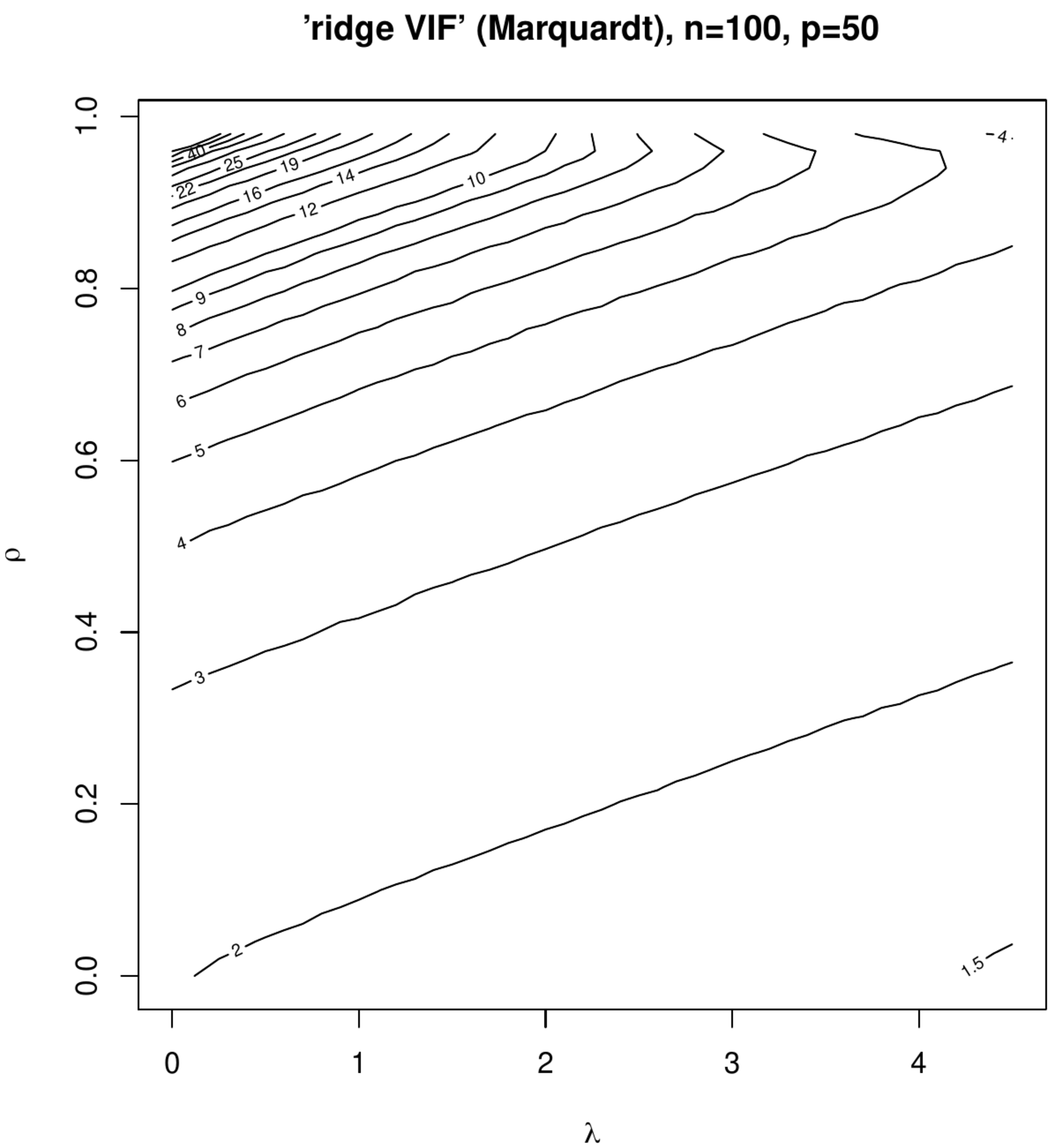
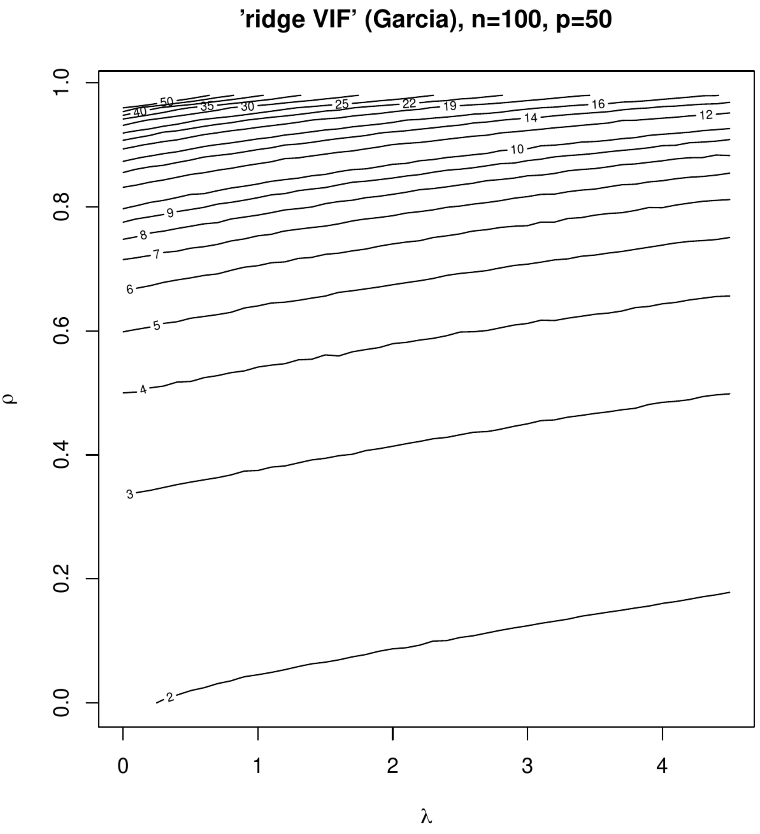
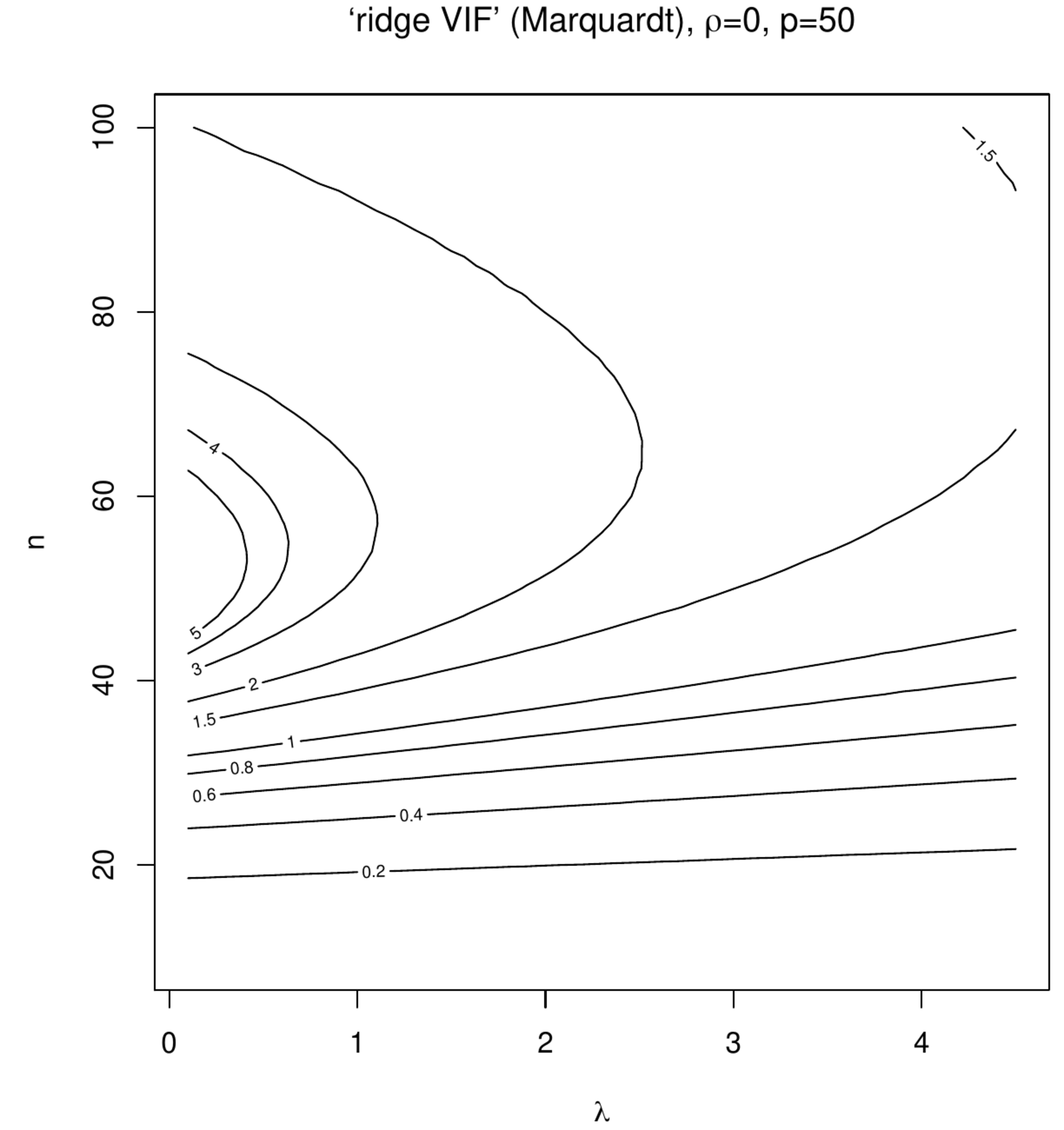
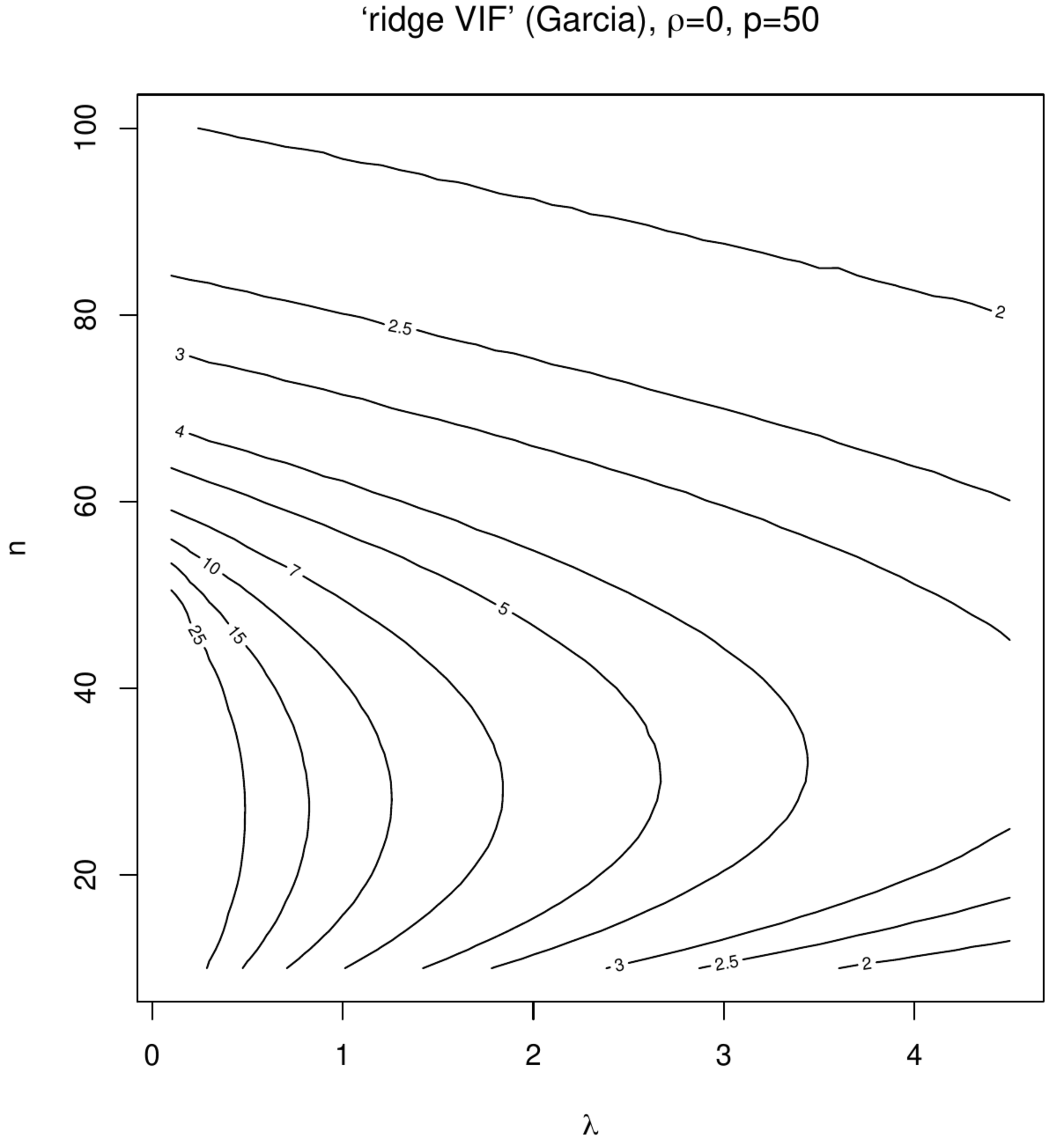
Contour plots of ‘Marquardt VIFs’ and ‘Garcia VIFs’, left and right columns, respectively. The top panels show these VIFs against the degree of penalization ([math]x[/math]-axis) and collinearity ([math]y[/math]-axis) for a fixed sample size ([math]n=100[/math]) and dimension ([math]p=50[/math]). The bottom panels show these VIFs against the degree of penalization ([math]x[/math]-axis) and the sample size ([math]y[/math]-axis) for a fixed dimension ([math]p=50[/math]).
An alternative definition of the ‘ridge VIF’ presented by [13] for the ‘[math]p=2[/math]’-case, which they motivate from counterintuitive behaviour observed in the ‘ridge VIF’ defined by [12], adopts the ‘maximum likelihood VIF’ definition but derives the ridge regression estimator from augmented data to comply with the maximum likelihood approach. This requires to augment the response vector with [math]p[/math] zeros, i.e. [math]\mathbf{Y}_{\mbox{{\tiny aug}}} = (\mathbf{Y}^{\top}, \mathbf{0}_p^{\top})^{\top}[/math] and the design matrix with [math]p[/math] rows as [math]\mathbf{X}_{\mbox{{\tiny aug}}} = (\mathbf{X}^{\top}, \sqrt{\lambda} \mathbf{I}_{pp})^{\top}[/math]. The ridge regression estimator can then be written as [math]\hat{\bbeta} (\lambda) = (\mathbf{X}_{\mbox{{\tiny aug}}}^{\top} \mathbf{X}_{\mbox{{\tiny aug}}})^{-1} \mathbf{X}_{\mbox{{\tiny aug}}}^{\top} \mathbf{Y}_{\mbox{{\tiny aug}}}[/math] (see Exercise). This reformulation of the ridge regression estimator in the form of its maximum likelihood counterpart suggests the adoption of latter's VIF definition for the former. However, in the ‘maximum likelihood VIF’ the design matrix is assumed to be zero centered column-wise. Within the augmented data formulation this may be achieved by the inclusion of a column of ones in [math]\mathbf{X}_{\mbox{{\tiny aug}}}[/math] representing the intercept. The inclusion of an intercept, however, requires a modification of the estimators of [math]\mbox{Var}(X_{i,j})[/math] and [math]\mbox{Var}(X_{i,j} \, | \, X_{i,1}, \ldots, X_{i,j-1}, X_{i,j+1}, \ldots, X_{i,p})[/math]. The former is readily obtained, %: [math](n+p)^{-1} \sum_{i=1}^{n+p} (X_{i,j} - (n+p)^{-1} \sqrt{\lambda})^2[/math]. while the latter is given by the reciprocals of the [math]2^{\mbox{{\tiny nd}}}[/math] to the [math](p+1)[/math]-th diagonal elements of the inverse of:
The lower right block of this inverse is obtained using well-known linear algebra results i) the analytic expression of the inverse of a [math]2\times 2[/math]-partitioned block matrix and i) the inverse of the sum of an invertible and a rank one matrix (given by the Sherman-Morrison formula, see Corollary 18.2.10, [14]). It equals:
where [math]c = (n+p)^{-1} \lambda \, \mathbf{1}_p^{\top} ( \mathbf{X}^{\top} \mathbf{X} + \lambda \mathbf{I}_{pp} )^{-1} \mathbf{1}_p = (n+p)^{-1} \lambda \sum_{j, j'=1}^p [( \mathbf{X}^{\top} \mathbf{X} + \lambda \mathbf{I}_{pp} )^{-1} ]_{j,j'}[/math]. Substitution of these expressions in the ratio of [math]\mbox{Var}(X_{i,j})[/math] and [math]\mbox{Var}(X_{i,j} \, | \, X_{i,1}, \ldots, X_{i,j-1}, X_{i,j+1}, \ldots, X_{i,p})[/math] in the above yields the alternative VIF of [13].
The effect of collinearity on the variance of the ridge regression estimator and the influence of penalization on this effect is studied in two small simulation studies. In the first study the rows of the design matrix [math]\mathbf{X}_{i,\ast}^{\top}[/math] are sampled from [math]\mathcal{N}(\mathbf{0}_p, \mathbf{\Sigma})[/math] with [math]\mathbf{\Sigma} = (1-\rho) \mathbf{I}_{pp} + \rho \mathbf{1}_{pp}[/math] fixing the dimension at [math]p=50[/math] and the sample size at [math]n=100[/math]. The correlation coefficient [math]\rho[/math] is varied over the unit interval [math][0,1)[/math], representing various levels of collinearity. The columns of the thus drawn [math]\mathbf{X}[/math] are zero centered. The response is then formed in accordance with the linear regression model [math]\mathbf{Y} = \mathbf{X} \bbeta + \vvarepsilon[/math] with [math]\bbeta = \mathbf{1}_{p}[/math] and the error drawn from [math]\mathcal{N}(\mathbf{0}_n, \tfrac{1}{4} \mathbf{I}_{nn})[/math]. The effect of penalization is studied by varying [math]\lambda[/math]. For each [math](\rho, \lambda)[/math]-combination data, [math]\mathbf{X}[/math] and [math]\mathbf{Y}[/math], are sampled thousand times and both ‘ridge VIFs’, for discriminative purposes referred as the Marquardt and Garcia VIFs (after the first author of the proposing papers), are calculated and averaged. Figure shows the contour plots of the averaged Marquardt and Garcia VIF against [math]\rho[/math] and [math]\lambda[/math]. At [math](\rho, \lambda) \approx (0, 0)[/math] both VIFs are close to two, which -- although the set-up is not high-dimensional in the strict ‘[math]p \gt n[/math]’-sense -- is due to the streneous [math]p/n[/math]-ratio. Nonetheless, as expected an increase in collinearity results in an increase in the VIF (irrespective of the type). Moreover, indeed some counterintuitive behaviour is observed in the Marquardt VIF: at (say) a value of [math]\lambda=3[/math] the VIF reaches a maximum for [math]\rho \approx 0.95[/math] and declines for larger degrees of collinearity. This is left without further interpretation as interest is not in deciding on the most appropriate operationalization among both VIFs of the ridge regression estimator, but is primarily in the effect of penalization on the VIF. In this respect both VIFs exhibit the same behaviour: a monotone decrease of both VIFs in [math]\lambda[/math].
In the second simulation the effect of ‘spurious collinearity’ introduced by the varying the sample size on the ridge estimator is studied. The settings are identical to that of the first simulation but with [math]\rho=0[/math] and a sample size [math]n[/math] that varies from ten to hundred. With [math]p=50[/math] in particular the lower sample sizes will exhibit high degrees of collinearity as the sample correlation coefficient has been seen to inflate then. % (as is pointed out by [15] and illustrated in Section \ref{sect:ridgeEstimator}). The resulting contour plots (Figure) now present the VIFs against [math]n[/math] and [math]\lambda[/math]. Although some counterintuitive behaviour can be seen around [math]n=p[/math] and small [math]\lambda[/math], the point to be noted and relevant here -- as interest is in the VIF's behaviour for data sets with a fixed sample size and covariates drawn without collinearity -- is the monotone decrease of both VIFs in [math]\lambda[/math] at any sample size.
In summary, the penalization does not remove collinearity but, irrespective of the choice of VIF, it reduces the effect of collinearity on the variance of the ridge estimator (as measured by the VIFs above). This led [13] -- although admittingly their focus appears to be low-dimensionally -- to suggest that the VIFs may guide the choice the penalty parameter: choose [math]\lambda[/math] such that the variance of the estimator is increased at most by a user-specified factor.
Illustration
The application of ridge regression to actual data aims to illustrate its use in practice.
MCM7 expression regulation by microRNAs
Recently, a new class of RNA was discovered, referred to as microRNA. MicroRNAs are non-coding, single stranded RNAs of approximately 22 nucleotides. Like mRNAs, microRNAs are encoded in and transcribed from the DNA. MicroRNAs play an important role in the regulatory mechanism of the cell. MicroRNAs down-regulate gene expression by either of two post-transcriptional mechanisms: mRNA cleavage or transcriptional repression. This depends on the degree of complementarity between the microRNA and the target. Perfect or nearly perfect complementarity of the mRNA to the microRNA will lead to cleavage and degradation of the target mRNA. Imperfect complementarity will repress the productive translation and reduction in protein levels without affecting the mRNA levels. A single microRNA can bind to and regulate many different mRNA targets. Conversely, several microRNAs can bind to and cooperatively control a single mRNA target ([16]; [17]; [18]).
In this illustration we wish to confirm the regulation of mRNA expression by microRNAs in an independent data set. We cherry pick an arbitrary finding from literature reported in [19], which focusses on the microRNA regulation of the MCM7 gene in prostate cancer. The MCM7 gene is involved in DNA replication [20], a cellular process often derailed in cancer. Furthermore, MCM7 interacts with the tumor-suppressor gene RB1 [21]. Several studies indeed confirm the involvement of MCM7 in prostate cancer [22]. And recently, it has been reported that in prostate cancer MCM7 may be regulated by microRNAs [19].
We here assess whether the MCM7 down-regulation by microRNAs can be observed in a data set other than the one upon which the microRNA-regulation of MCM7 claim has been based. To this end we download from the Gene Expression Omnibus (GEO) a prostate cancer data set (presented by [23]). This data set (with GEO identifier: GSE20161) has both mRNA and microRNA profiles for all samples available. The preprocessed (as detailed in [23]) data are downloaded and require only minor further manipulations to suit our purpose. These manipulations comprise
- averaging of duplicated profiles of several samples,
- gene- and mir-wise zero-centering of the expression data,
- averaging the expression levels of the probes that interrogate MCM7. Eventually, this leaves 90 profiles each comprising of 735 microRNA expression measurements.
# load libraries
library(GEOquery)
library(RmiR.hsa)
library(penalized)

# extract data
slh     <- getGEO("GSE20161", GSEMatrix=TRUE)
GEdata  <- slh[1][[1]]
MIRdata <- slh[2][[1]]

# average duplicate profiles
Yge  <- numeric()
Xmir <- numeric()
for (sName in 1:90){
	Yge  <- cbind(Yge,  apply(exprs(GEdata)[,sName,drop=FALSE],  1, mean))
	Xmir <- cbind(Xmir, apply(exprs(MIRdata)[,sName,drop=FALSE], 1, mean))
}
colnames(Yge)  <- paste("S", 1:90, sep="")
colnames(Xmir) <- paste("S", 1:90, sep="")

# extact mRNA expression of the MCM7N tumor suppressor gene
entrezID <- c("4176")
geneName <- "MCM7"
Y        <- Yge[which(fData(GEdata)[,10] == entrezID),]

# average gene expression levels over probes
Y <- apply(Y, 2, mean)

# mir-wise centering mir expression data
X <- t(sweep(Xmir, 1, rowMeans(Xmir)))

# generate cross-validated likelihood profile
profL2(Y, penalized=X, minlambda2=1, maxlambda2=20000, plot=TRUE)

# decide on the optimal penalty value directly
optLambda <- optL2(Y, penalized=X)$lambda

# obtain the ridge regression estimages
ridgeFit <- penalized(Y, penalized=X, lambda2=optLambda)

# plot them as histogram
hist(coef(ridgeFit, "penalized"), n=50, col="blue", border="lightblue",
     xlab="ridge regression estimates with optimal lambda",
     main="Histogram of ridge estimates")

#  linear prediction from ridge
Yhat <- predict(ridgeFit, X)[,1]
plot(Y ~ Yhat, pch=20, xlab="pred. MCM7 expression",
                       ylab="obs. MCM7 expression")
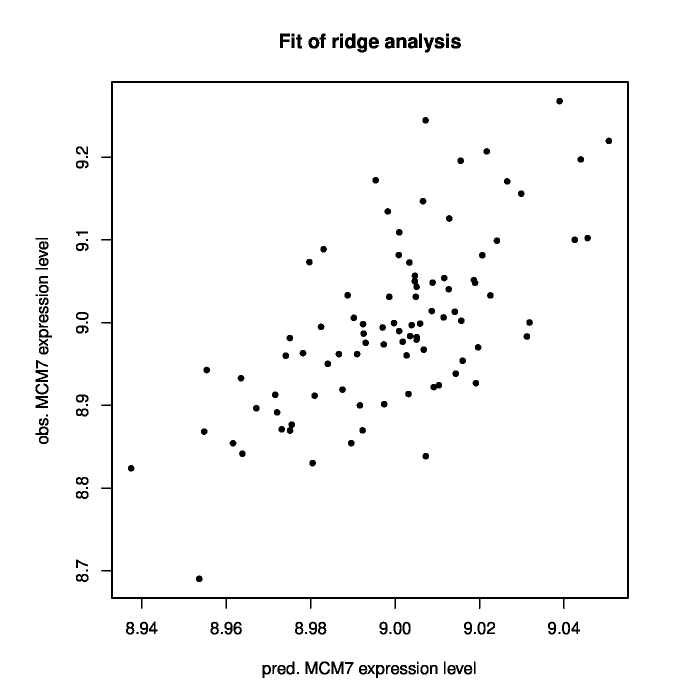
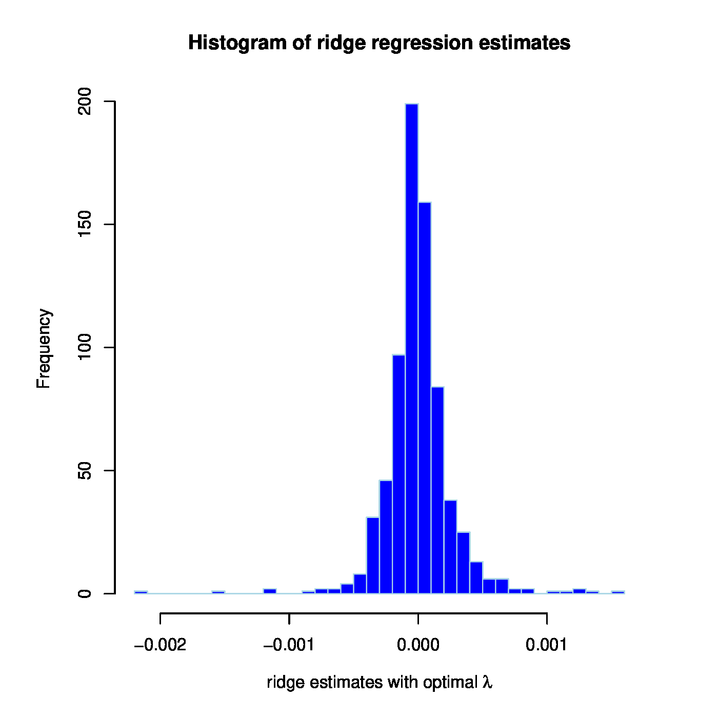
With this prostate data set at hand we now investigate whether MCM7 is regulated by microRNAs. Hereto we fit a linear regression model regressing the expression levels of MCM7 onto those of the microRNAs. As the number of microRNAs exceeds the number of samples, ordinary least squares fails and we resort to the ridge estimator of the regression coefficients. First, an informed choice of the penalty parameter is made through maximization of the LOOCV log-likelihood, resulting in [math]\lambda_{\mbox{{\tiny opt}}} = 1812.826[/math]. Having decided on the value of the to-be-employed penalty parameter, the ridge regression estimator can now readily be evaluated. The thus fitted model allows for the evaluation of microRNA-regulation of MCM7. E.g., by the proportion of variation of the MCM7 expression levels by the microRNAs as expressed in coefficient of determination: [math]R^2 = 0.4492[/math]. Alternatively, but closely related, observed expression levels may be related to the linear predictor of the MCM7 expression levels: [math]\hat{\mathbf{Y}}(\lambda_{\mbox{{\tiny opt}}}) = \mathbf{X} \hat{\bbeta} (\lambda_{\mbox{{\tiny opt}}})[/math]. The Spearman correlation of response and predictor equals 0.6295. A visual inspection is provided by the left panel of Figure. Note the difference in scale of the [math]x[/math]- and [math]y[/math]-axes. This is due to the fact that the regression coefficients have been estimated in penalized fashion, consequently shrinking estimates of the regression coefficients towards zero leading to small estimates and in turn compressing the range of the linear prediction. The above suggests there is indeed association between the microRNA expression levels and those of MCM7.
Left panel: Observed vs. (ridge) fitted MCM7 expression values. Right panel: Histogram of the ridge regression coefficient estimates.
The overall aim of this illustration was to assess whether microRNA-regulation of MCM7 could also be observed in this prostate cancer data set. In this endeavour the dogma (stating this regulation should be negative) has nowhere been used. A first simple assessment of the validity of this dogma studies the signs of the estimated regression coefficients. The ridge regression estimate has 394 out of the 735 microRNA probes with a negative coefficient. Hence, a small majority has a sign in line with the ‘microRNA [math]\downarrow[/math] mRNA’ dogma. When, in addition, taking the size of these coefficients into account (Figure, right panel), the negative regression coefficient estimates do not substantially differ from their positive counterparts (as can be witnessed from their almost symmetrical distribution around zero). Hence, the value of the ‘microRNA [math]\downarrow[/math] mRNA’ dogma is not confirmed by this ridge regression analysis of the MCM7-regulation by microRNAs. Nor is it refuted.
The implementation of ridge regression in the penalized-package offers the possibility to fully obey the dogma on negative regulation of mRNA expression by microRNAs. This requires all regression coefficients to be negative. Incorporation of the requirement into the ridge estimation augments the constrained estimation problem with an additional constraint:
With the additional non-positivity constraint on the parameters, there is no explicit solution for the estimator. The ridge estimate of the regression parameters is then found by numerical optimization using e.g. the Newton-Raphson algorithm or a gradient descent approach. The next listing gives the R-code for ridge estimation with the non-positivity constraint of the linear regression model.
# decide on the optimal penalty value with sign constraint on paramers
optLambda <- optL2(Y, penalized=-X, positive=rep(TRUE, ncol(X)))$lambda

# obtain the ridge regression estimages
ridgeFit <- penalized(Y, penalized=-X, lambda2=optLambda,
                      positive=rep(TRUE, ncol(X)))

#  linear prediction from ridge
Yhat <- predict(ridgeFit, -X)[,1]
plot(Y ~ Yhat, pch=20, xlab="predicted MCM7 expression level",
                       ylab="observed MCM7 expression level")
cor(Y, Yhat, m="s")
summary(lm(Y ~ Yhat))[8]
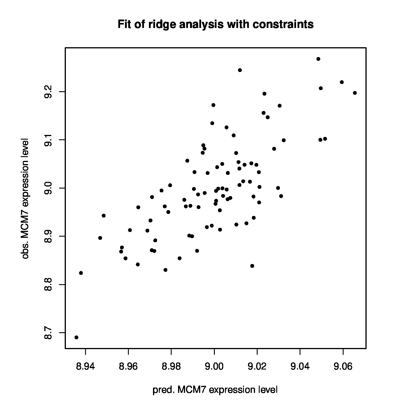
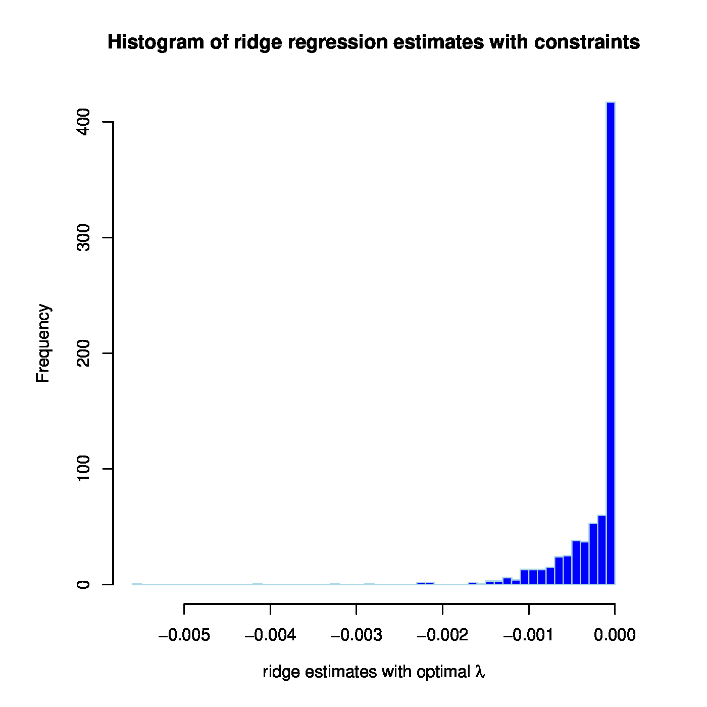
The linear regression model linking MCM7 expression to that of the microRNAs is fitted by ridge regression while simultaneously obeying the ‘negative regulation of mRNA by microRNA’-dogma to the prostate cancer data. In the resulting model 401 out of 735 microRNA probes have a nonzero (and negative) coefficient. There is a large overlap in microRNAs with a negative coefficient between those from this and the previous fit. The models are also compared in terms of their fit to the data. The Spearman rank correlation coefficient between response and predictor for the model without positive regression coefficients equals 0.679 and its coefficient of determination 0.524 (confer the left panel of Figure for a visualization). This is a slight improvement upon the unconstrained ridge estimated model. The improvement may be small but it should be kept in mind that the number of parameters used by both models is 401 (for the model without positive regression coefficients) vs. 735. Hence, with close to half the number of parameters the dogma-obeying model gives a somewhat better description of the data. This may suggest that there is some value in the dogma as inclusion of this prior information leads to a more parsimonious model without any loss in fit.
Left panel: Observed vs. (ridge) fitted MCM7 expression values (with the non-positive constraint on the parameters in place). Right panel: Histogram of the ridge regression coefficient estimates (from the non-positivity constrained analysis).
The dogma-obeying model selects 401 microRNAs that aid in the explanation of the variation in the gene expression levels of MCM7. There is an active field of research, called target prediction, trying to identify which microRNAs target the mRNA of which genes. Within R there is a collection of packages that provide the target prediction of known microRNAs. The packages differ on the method (e.g. experimental or sequence comparison) that has been used to arrive at the prediction. These target predictions may be used to evaluate the value of the found 401 microRNAs. Ideally, there would be a substantial amount of overlap. The R-script that loads the target predictions and does the comparison is below.
# extract mir names and their (hypothesized) mrna target
mir2target     <- numeric()
mirPredProgram <- c("targetscan", "miranda", "mirbase", "pictar", "mirtarget2")
for (program in mirPredProgram){
    slh           <- dbReadTable(RmiR.hsa_dbconn(), program)
    slh           <- cbind(program, slh[,1:2])
    colnames(slh) <- c("method", "mir", "target")
    mir2target    <- rbind(mir2target, slh)
}
mir2target <- unique(mir2target)
mir2target <- mir2target[which(mir2target[,3] == entrezID),]
uniqMirs   <- tolower(unique(mir2target[,2]))

# extract names of mir-probe on array
arrayMirs <- tolower(levels(fData(MIRdata)[,3])[fData(MIRdata)[,3]])

# which mir-probes are predicted to down-regulate MCM7
selMirs <- intersect(arrayMirs, uniqMirs)
ids     <- which(arrayMirs %in% selMirs)

# which ridge estimates are non-zero
nonzeroBetas <- (coef(ridgeFit, "penalized") != 0)

# which mirs are predicted to
nonzeroPred      <- 0 * betas
nonzeroPred[ids] <- 1

# contingency table and chi-square test
table(nonzeroBetas, nonzeroPred)
chisq.test(table(nonzeroBetas, nonzeroPred))
| [math]\hat{\beta}_j = 0[/math] | [math]\hat{\beta}_j \lt 0[/math] | |
| microRNA not target | 323 | 390 |
| microRNA target | 11 | 11 |
With knowledge available on each microRNA whether it is predicted (by at least one target prediction package) to be a potential target of MCM7, it may be cross-tabulated against its corresponding regression coefficient estimate in the dogma-obeying model being equal to zero or not. Table contains the result. Somewhat superfluous considering the data, we may test whether the targets of MCM7 are overrepresented in the group of strictly negatively estimated regression coefficients. The corresponding chi-squared test (with Yates' continuity correction) yields the test statistic [math]\chi^2 = 0.0478[/math] with a [math]p[/math]-value equal to 0.827. Hence, there is no enrichment among the 401 microRNAS of those that have been predicted to target MCM7. This may seem worrisome. However, the microRNAs have been selected for their predictive power of the expression levels of MCM7. Variable selection has not been a criterion (although the sign constraint implies selection). Moreover, criticism on the value of the microRNA target prediction has been accumulating in recent years (REF).
Conclusion
We discussed ridge regression as a modification of linear regression to overcome the empirical non-identifiability of the latter when confronted with high-dimensional data. The means to this end was the addition of a (ridge) penalty to the sum-of-squares loss function of the linear regression model, which turned out to be equivalent to constraining the parameter domain. This warranted the identification of the regression coefficients, but came at the cost of introducing bias in the estimates. Several properties of ridge regression like moments and its MSE have been reviewed. Finally, its behaviour and use have been illustrated in simulation and omics data.
General References
van Wieringen, Wessel N. (2021). "Lecture notes on ridge regression". arXiv:1509.09169 [stat.ME].
References
- 1.0 1.1 Peeters, C. F. W., van de Wiel, M. A., and van Wieringen, W. N. (2019).The spectral condition number plot for regularization parameter evaluation.Computational Statistics, 35, 629--646
- Saleh, A. K. M. E., Arashi, M., and Kibria, B. M. G. (2019).Theory of ridge regression estimation with applications, volume 285.John Wiley & Sons
- Akaike, H. (1974).A new look at the statistical model identification.IEEE Transactions on Automatic Control, 19(6), 716--723
- Schwarz, G. (1978).Estimating the dimension of a model.Annals of Statistics, 6(2), 461--464
- Allen, D. M. (1974).The relationship between variable selection and data agumentation and a method for prediction.Technometrics, 16(1), 125--127
- 6.0 6.1 6.2 Golub, G. H., Heath, M., and Wahba, G. (1979).Generalized cross-validation as a method for choosing a good ridge parameter.Technometrics, 21(2), 215--223
- van de Wiel, M. A., van Nee, M. M., and Rauschenberger, A. (2021).Fast cross-validation for multi-penalty ridge regression.Journal of Computational and Graphical Statistics, (just-accepted), 1--31
- Li, K.-C. (1986).Asymptotic optimality of [math]c\_l[/math] and generalized cross-validation in ridge regression with application to spline smoothing.The Annals of Statistics, 14(3), 1101--1112
- Sardy, S. (2008).On the practice of rescaling covariates.International Statistical Review, 76(2), 285--297
- Mathai, A. M. and Provost, S. B. (1992).Quadratic Forms in Random Variables: Theory and Applications.Dekker
- Whittaker, J. (1990).Graphical Models in Applied Multivariate Statistics.John Wiley & Sons, Chichester, England
- 12.0 12.1 Marquardt, D. W. (1970).Generalized inverses, ridge regression and biased linear estimation. technometrics, 12.Technometrics, 12, 591--612
- 13.0 13.1 13.2 García, C. B., García, J., López Martín, M., and Salmerón, R. (2015).Collinearity: Revisiting the variance inflation factor in ridge regression.Journal of Applied Statistics, 42(3), 648--661
- Harville, D. A. (2008).Matrix Algebra From a Statistician's Perspective.Springer, New York
- Cite error: Invalid
<ref>tag; no text was provided for refs namedHero2012 - Bartel, D. P. (2004).MicroRNAs: genomics, biogenesis, mechanism, and function.Cell, 116(2), 281--297
- Esquela-Kerscher, A. and Slack, F. J. (2006).Oncomirs: microRNAs with a role in cancer.Nature Reviews Cancer, 6(4), 259--269
- Kim, V. N. and Nam, J.-W. (2006).Genomics of microRNA.TRENDS in Genetics, 22(3), 165--173
- 19.0 19.1 Ambs, S., Prueitt, R. L., Yi, M., Hudson, R. S., Howe, T. M., Petrocca, F., Wallace, T. A., Liu, C.-G., Volinia, S., Calin, G. A., Yfantis, H. G., Stephens, R. M., and Croce, C. M. (2008).Genomic profiling of microrna and messenger RNA reveals deregulated microrna expression in prostate cancer.Cancer Research, 68(15), 6162--6170
- Tye, B. K. (1999).MCM proteins in DNA replication.Annual Review of Biochemistry, 68(1), 649--686
- Sterner, J. M., Dew-Knight, S., Musahl, C., Kornbluth, S., and Horowitz, J. M. (1998).Negative regulation of DNA replication by the retinoblastoma protein is mediated by its association with MCM7.Molecular and Cellular Biology, 18(5), 2748--2757
- Padmanabhan, V., Callas, P., Philips, G., Trainer, T., and Beatty, B. (2004).DNA replication regulation protein MCM7 as a marker of proliferation in prostate cancer.Journal of Clinical Pathology, 57(10), 1057--1062
- 23.0 23.1 Wang, L., Tang, H., Thayanithy, V., Subramanian, S., Oberg, L., Cunningham, J. M., Cerhan, J. R., Steer, C. J., and Thibodeau, S. N. (2009).Gene networks and microRNAs implicated in aggressive prostate cancer.Cancer research, 69(24), 9490--9497
