Survival Analysis

Survival analysis is a branch of statistics for analyzing the expected duration of time until one event occurs, such as death in biological organisms and failure in mechanical systems. Survival analysis attempts to answer certain questions, such as what is the proportion of a population which will survive past a certain time? Of those that survive, at what rate will they die or fail? Can multiple causes of death or failure be taken into account? How do particular circumstances or characteristics increase or decrease the probability of survival?

To answer such questions, it is necessary to define "lifetime". In the case of biological survival, death is unambiguous, but for mechanical reliability, failure may not be well-defined, for there may well be mechanical systems in which failure is partial, a matter of degree, or not otherwise localized in time. Even in biological problems, some events (for example, heart attack or other organ failure) may have the same ambiguity. The theory outlined below assumes well-defined events at specific times; other cases may be better treated by models which explicitly account for ambiguous events.

More generally, survival analysis involves the modelling of time to event data; in this context, death or failure is considered an "event" in the survival analysis literature – traditionally only a single event occurs for each subject, after which the organism or mechanism is dead or broken. Recurring event or repeated event models relax that assumption. The study of recurring events is relevant in systems reliability, and in many areas of social sciences and medical research.

Survival Function

The survival function is a function that gives the probability that a patient, device, or other object of interest will survive past a certain time. The survival function is also known as the survivor function or reliability function. The term reliability function is common in engineering while the term survival function is used in a broader range of applications, including human mortality. The survival function is the complementary cumulative distribution function of the lifetime. Sometimes complementary cumulative distribution functions are called survival functions in general.

Definition

Let the lifetime [math]T[/math] be a continuous random variable with cumulative hazard function [math]F(t)[/math] and hazard function [math]f(t)[/math] on the interval [math][0,\infty)[/math]. Its survival function or reliability function is:

[[math]]S(t) = P(\{T \gt t\}) = \int_t^{\infty} f(u)\,du = 1-F(t).[[/math]]

Examples of survival functions

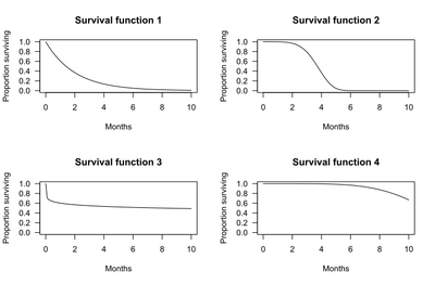
The graphs below show examples of hypothetical survival functions. The x-axis is time. The y-axis is the proportion of subjects surviving. The graphs show the probability that a subject will survive beyond time t.

Four survival functions

For example, for survival function 1, the probability of surviving longer than t = 2 months is 0.37. That is, 37% of subjects survive more than 2 months.

Survival function 1

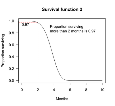
For survival function 2, the probability of surviving longer than t = 2 months is 0.97. That is, 97% of subjects survive more than 2 months.

Survival function 2

Median survival may be determined from the survival function: The median survival is the point where the survival function intersects the value 0.5. For example, for survival function 2, 50% of the subjects survive 3.72 months. Median survival is thus 3.72 months.

Survival function with indicated median survival

In some cases, median survival cannot be determined from the graph. For example, for survival function 4, more than 50% of the subjects survive longer than the observation period of 10 months.

Median survival greater than 10 months

The survival function is one of several ways to describe and display survival data. Another useful way to display data is a graph showing the distribution of survival times of subjects. Olkin, page 426, gives the following example of survival data. The number of hours between successive failures of an air-conditioning system were recorded. The time between successive failures are 1, 3, 5, 7, 11, 11, 11, 12, 14, 14, 14, 16, 16, 20, 21, 23, 42, 47, 52, 62, 71, 71, 87, 90, 95, 120, 120, 225, 246, and 261 hours. The mean time between failures is 59.6. This mean value will be used shortly to fit a theoretical curve to the data. The figure below shows the distribution of the time between failures. The blue tick marks beneath the graph are the actual hours between successive failures.

Distribution of AC failure times

The distribution of failure times is over-laid with a curve representing an exponential distribution. For this example, the exponential distribution approximates the distribution of failure times. The exponential curve is a theoretical distribution fitted to the actual failure times. This particular exponential curve is specified by the parameter lambda, λ= 1/(mean time between failures) = 1/59.6 = 0.0168. The distribution of failure times is called the probability density function (pdf), if time can take any positive value. In equations, the pdf is specified as f(t). If time can only take discrete values (such as 1 day, 2 days, and so on), the distribution of failure times is called the probability mass function (pmf). Most survival analysis methods assume that time can take any positive value, and f(t) is the pdf. If the time between observed air conditioner failures is approximated using the exponential function, then the exponential curve gives the probability density function, f(t), for air conditioner failure times.

Another useful way to display the survival data is a graph showing the cumulative failures up to each time point. These data may be displayed as either the cumulative number or the cumulative proportion of failures up to each time. The graph below shows the cumulative probability (or proportion) of failures at each time for the air conditioning system. The stairstep line in black shows the cumulative proportion of failures. For each step there is a blue tick at the bottom of the graph indicating an observed failure time. The smooth red line represents the exponential curve fitted to the observed data.

CDF for AC failures

A graph of the cumulative probability of failures up to each time point is called the cumulative distribution function, or CDF. In survival analysis, the cumulative distribution function gives the probability that the survival time is less than or equal to a specific time, t.

Let [math]T[/math] be survival time, which is any positive number. A particular time is designated by the lower case letter [math]t[/math]. The cumulative distribution function of [math]T[/math] is the function

[[math]]F(t) = \operatorname{P}(T\leq t),[[/math]]

where the right-hand side represents the probability that the random variable [math]T[/math] is less than or equal to [math]t[/math]. If time can take on any positive value, then the cumulative distribution function [math]F(t)[/math] is the integral of the probability density function [math]f(t)[/math].

For the air conditioning example, the graph of the CDF below illustrates that the probability that the time to failure is less than or equal to 100 hours is 0.81, as estimated using the exponential curve fit to the data.

AC Time to failure LT 100 hours

An alternative to graphing the probability that the failure time is less than or equal to 100 hours is to graph the probability that the failure time is greater than 100 hours. The probability that the failure time is greater than 100 hours must be 1 minus the probability that the failure time is less than or equal to 100 hours, because total probability must sum to 1.

This gives

[[math]] P(\textrm{failure time} \gt 100 \, \textrm{hours}) = 1 - P(\textrm{failure time} \lt 100 \, \textrm{hours}) = 1 – 0.81 = 0.19. [[/math]]

This relationship generalizes to all failure times:

[[math]] P(T \gt t) = 1 - P(T \lt t) = 1 – \textrm{cumulative distribution function}. [[/math]]

This relationship is shown on the graphs below. The graph on the left is the cumulative distribution function, which is [math]P(T \lt t)[/math]. The graph on the right is [math]P(T \gt t) = 1 - P(T \lt t)[/math]. The graph on the right is the survival function, [math]S(t)[/math]. The fact that the [math]S(t) = 1 – CDF[/math] is the reason that another name for the survival function is the complementary cumulative distribution function.

Survival function is 1 - CDF

Force of Mortality

In actuarial science, force of mortality represents the instantaneous rate of mortality at a certain age measured on an annualized basis. It is identical in concept to failure rate, also called hazard function, in reliability theory.

Motivation and definition

In a life table, we consider the probability of a person dying from age [math]x[/math] to [math]x + 1[/math], called [math]q_x[/math]. In the continuous case, we could also consider the conditional probability of a person who has attained age ([math]x[/math]) dying between ages [math]x[/math] and [math]x + \Delta x[/math], which is

[[math]]P_{x}(\Delta x)=P(x \lt X \lt x+\Delta\;x\mid\;X \gt x)=\frac{F_X(x+\Delta\;x)-F_X(x)}{(1-F_X(x))}[[/math]]

where [math]F_X[/math] is the cumulative distribution function of the continuous age-at-death random variable, [math]X[/math]. As [math]\Delta x[/math] tends to zero, so does this probability in the continuous case. The approximate force of mortality is this probability divided by [math]\Delta x[/math]. If we let [math]\Delta x[/math] tend to zero, we get the function for force of mortality, denoted by [math]\mu(x)[/math]:

[[math]]\mu\,(x)= \lim_{\Delta x \rightarrow 0} \frac{F_X(x+\Delta\;x)-F_X(x)}{\Delta x (1-F_X(x))} = \frac{F'_X(x)}{1-F_X(x)}[[/math]]

Since [math]f_X(x) = F'_X(x)[/math] is the probability density function of [math]X[/math], and [math]S(x)= 1 - F_X(x)[/math] is the survival function, the force of mortality can also be expressed variously as:

[[math]]\mu\,(x)=\frac{f_X(x)}{1-F_X(x)}=-\frac{S'(x)}{S(x)}=-{\frac{d}{dx}}\ln[S(x)].[[/math]]

To understand conceptually how the force of mortality operates within a population, consider that the ages, [math]x[/math], where the probability density function [math]f_X(x)[/math], there is no chance of dying. Thus the force of mortality at these ages is zero. The force of mortality [math]\mu(x)[/math] uniquely defines a probability density function [math]f_X(x)[/math].

The force of mortality [math]\mu(x)[/math] can be interpreted as the conditional density of failure at age [math]x[/math], while [math]f(x)[/math] is the unconditional density of failure at age [math]x[/math]. The unconditional density of failure at age [math]x[/math] is the product of the probability of survival to age [math]x[/math], and the conditional density of failure at age [math]x[/math], given survival to age [math]x[/math].

This is expressed in symbols as

[[math]]\,\mu(x)S(x) = f_X(x)[[/math]]

or equivalently

[[math]]\mu(x) = \frac{f_X(x)}{S(x)}.[[/math]]

In many instances, it is also desirable to determine the survival probability function when the force of mortality is known. To do this, integrate the force of mortality over the interval [math]x[/math] to [math]x + t[/math]

[[math]] \int_{x}^{x+t} \mu(y) \, dy = \int_{x}^{x+t} -\frac{d}{dy} \ln[S(y)]\, dy [[/math]]

.

By the fundamental theorem of calculus, this is simply

[[math]] -\int_{x}^{x+t} \mu(y) \, dy = \ln[S(x + t)] - \ln[S(x)]. [[/math]]

Let us denote

[[math]] S_x(t) = \frac{S(x+t)}{S(x)}, [[/math]]

then taking the exponent to the base e, the survival probability of an individual of age [math]x[/math] in terms of the force of mortality is

[[math]] S_x(t) = \exp \left(-\int_x^{x+t}\mu(y)\, dy\, \right). [[/math]]

Examples

Type	Force of mortality	Survival function
Exponential	[[math]]\mu(y) = \lambda[[/math]]	[[math]]S_x(t) = e^{-\int_x^{x+t} \lambda dy} = e^{-\lambda t}[[/math]]
Gamma	[[math]]\mu(y) = \frac{y^{\alpha-1} e^{-y}}{\Gamma(\alpha) - \gamma(\alpha, y)}, [[/math]]	[[math]]f(x) = \frac{x^{\alpha - 1} e^{-x}}{\Gamma(\alpha)}[[/math]]
Weibull	[[math]] \mu(y) = \alpha \lambda^\alpha y^{\alpha-1},[[/math]]	[[math]]S_x(t) = e^{-\int_x^{x+t}\mu(y) dy} = A(x) e^{ - (\lambda (x+t))^\alpha }, [[/math]] where [math]A(x) = e^{(\lambda x)^{\alpha}}.[/math]

Future lifetime of a life aged [math]x[/math]

Now, we extend our discussion from future lifetime of a life aged zero (a newborn) to a life aged [math] x[/math] ([math] x\ge 0[/math]). For simplicity of presentation, we denote a life aged [math] x[/math] by [math](x)[/math].

When we say "a life aged [math] x[/math]", we mean the life is aged exactly [math] x[/math], i.e. the life just reaches age [math] x[/math] (birthday of the life), but not, say aged [math] x+0.5[/math], [math] x+0.9[/math], etc, which are usually also referred as "aged [math] x[/math]" in our daily life.

Similarly, we denote the future lifetime of [math](x)[/math] by [math] t_x[/math] (recall that we denote the future lifetime of [math](0)[/math] (newborn) by [math] t_0[/math]). We define the distribution of [math] t_x[/math] mathematically (and quite naturally) as the conditional distribution of [math] t_0-x[/math], given that [math] t_0 \gt x[/math].

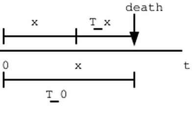
Refer to the following timeline:

We can observe that [math] t_x=T_0-x[/math] if [math] t_0 \gt x[/math] (or [math] t_0\ge x[/math], but since [math] t_0[/math] is continuous, it does not matter). So, if [math] t_0 \gt x[/math], then [math] t_x=T_0-x[/math].

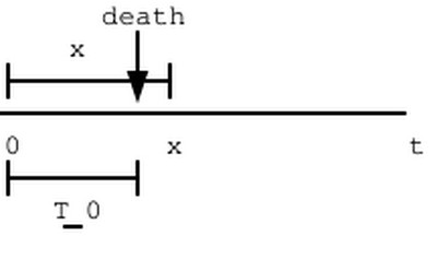
On the other hand, if [math] t_0 \lt x[/math], we have the following timeline:

In this case, [math] t_x[/math] does not exist, since the person does not survive for [math] x[/math] years, and thus will never be age [math] x[/math], so there is not [math](x)[/math], and therefore there is not [math] t_x[/math], future lifetime of [math](x)[/math]. This shows the necessity of the condition [math] t_0 \gt x[/math].

From this definition, we have [math]\mathbb P(T_x\le t)=\mathbb P(T_0-x\le t|T_0 \gt x)[/math], [math]\mathbb P(T_x \gt t)=\mathbb P(T_0-x \gt t|T_0 \gt x)[/math], etc.. This is quite important since it is the basis for the calculations of probabilities related to [math] t_x[/math].

For the pdf, cdf and survival function of [math] t_x[/math], we have similar notations as follows:

• [math]f_x(t)[/math]: pdf of [math] t_x[/math]
• [math]F_x(t)[/math]: cdf of [math] t_x[/math]
• [math]S_x(t)[/math]: survival function of [math] t_x[/math]

In particular, we have some special actuarial notations for the cdf and survival function, as follows:

• [math]_tq_x=F_x(t)=\mathbb P(T_x\le t)[/math]
• [math]_tp_x=S_x(t)=\mathbb P(T_x \gt t)=1-{}_tq_x[/math]

In actuarial notations, "[math]q[/math]" often refers to something related to death, while "[math]p[/math]" often refers to something related to survival. In this context, this holds since [math]_tq_x[/math] refers to the probability for [math](x)[/math] to die within [math] t[/math] time units, and [math]_tp_x[/math] refers to the probability for [math](x)[/math] to survive for [math] t[/math] time units.

For simplicity, if [math] t=1[/math], we write [math]_1q_x[/math] as [math]q_x[/math] and [math]_1p_x[/math] as [math]p_x[/math].

Using the relationship between [math] t_x[/math] and [math] t_0[/math], we can develop some useful formulas for [math]_tp_x[/math] and [math]_tq_x[/math], as follows:

Proposition

[[math]]_tp_x=\frac{S_0(t+x)}{S_0(x)}[[/math]]

and

[[math]]_tq_x=1-\frac{S_0(t+x)}{S_0(x)}.[[/math]]

Show Proof

First, we have [math]_tp_x=\mathbb P(T_x \gt t)=\mathbb P(T_0-x \gt t|T_0 \gt x)=\frac{\mathbb P(T_0 \gt t+x\cap T_0 \gt x)}{\mathbb P(T_0 \gt x)}=\frac{\mathbb P(T_0 \gt t+x)}{\mathbb P(T_0 \gt x)}=\frac{S_0(t+x)}{S_0(x)}[/math], in which [math]\{T_0 \gt t+x\}\cap \{T_0 \gt x\}=\{T_0 \gt t+x\}[/math] since [math] t+x \gt x[/math] ([math] t\ge 0[/math]), and so [math] t_0 \gt t+x\implies T_0 \gt x[/math], and thus [math]\{T_0 \gt t+x\}[/math] is a subset of [math]\{T_0 \gt x\}[/math].

It follows that [math]_tq_x=1-{}_tp_x=1-\frac{S_0(t+x)}{S_0(x)}[/math].

■

We can also express the pdf of [math] t_x[/math] as follows:

Proposition

[[math]]f_x(t)={}_xp_t\mu_{x+t}.[[/math]]

Show Proof

We have

[[math]]f_x(t)=\frac{d}{dt}{}_tq_x=\left(1-\frac{S_0(t+x)}{S_0(x)}\right)'=\frac{-S'_0(t+x)}{S_0(x)}=\frac{{\color{darkgreen}S_0(t+x)}}{S_0(x)}\cdot\frac{-S'_0(t+x)}{{\color{darkgreen}S_0(t+x)}}={}_tp_x\mu_{x+t}.[[/math]]

■

Intuitively (and roughly), [math]_tp_x[/math] gives the probability for [math](x)[/math] to survive for [math] t[/math] time units and after that, [math](x)[/math] becomes [math](x+t)[/math], and [math]\mu_{x+t}[/math] gives the probability for [math](x+t)[/math] to die "instantaneously" at time [math] x+t[/math], given that the person survives to [math] x+t[/math] time units. Multiplying [math]_tp_x[/math] and [math]\mu_{x+t}[/math], it means the same as the (rough) interpretation of [math]f_x(t)[/math]: [math](x)[/math] die very shortly after (or "exactly at") time [math] x+t[/math].

Example

It is given that the survival function of newborn is [math]S_0(t)=1-\frac{t}{10},\quad 0\le t\le 10[/math].

(a) Calculate [math]_2 p_1[/math] and [math]q_2[/math]. Hence, determine whether [math]_2 p_1=p_2[/math].

(b) Calculate [math]\mu_3[/math]. Hence, calculate [math]f_2(1)[/math].

Solution:

(a) [math]_2p_1=\frac{S_0(3)}{S_0(1)}=\frac{0.7}{0.9}\approx 0.778[/math] and [math]q_2=1-\frac{S_0(3)}{S_0(2)}=1-\frac{0.7}{0.8}=0.125[/math]. Since [math]p_2=1-q_2=0.875[/math], [math]_2p_1\ne p_2[/math].

(b) Since [math]S'_0(t)=-\frac{1}{10}[/math], [math]\mu_3=\frac{-S'_0(3)}{S_0(3)}=\frac{-(-1/10)}{0.7}\approx\frac{1}{7}[/math]. So, [math]f_2(1)={}_1p_2\mu_3=(0.875)(1/7)=0.125[/math].

We have a special notation for the probability for [math](x)[/math] to die between ages [math] x+t[/math] and [math] x+t+u[/math] ([math] x,t,u\ge 0[/math]), namely [math]_{t|u}q_x[/math] (we use "[math]q[/math]" here since this is related to death). Thus, we have by definition [math]_{t|u}q_x=\mathbb P(t \lt t_x \lt t+u))[/math]. We have the following proposition for another formula of [math]_{t|u}q_x[/math].

Proposition

[[math]]_{t|u}q_x={}_tp_x({}_uq_{x+t})[[/math]]

Show Proof

[[math]] \begin{align} _{t|u}q_x&=\mathbb P(t \lt t_x \lt t+u)\\ &=\mathbb P(T_x\le t+u)-\mathbb P(T_x\le t)\\ &={}_{t+u}q_x-_tq_x\\ &=(1-_{t+u}p_x)-(1-_tp_x)\\ &={}_tp_x-_{t+u}p_x\\ &={}_tp_x-\frac{S_0(x+t+u)}{S_0(x)}\\ &={}_tp_x-\frac{S_0(x+t+u)}{{\color{darkgreen}S_0(x+t)}}\left(\frac{{\color{darkgreen}S_0(x+t)}}{S_0(x)}\right)\\ &={}_tp_x-{}_up_{x+t}({}_tp_x)\\ &={}_tp_x(1-{}_up_{x+t})\\ &={}_tp_x(_uq_{x+t})\\ \end{align} [[/math]]

■

• For proving formulas like this, it is generally better to change all "[math]q[/math]" to "[math]p[/math]" in the intermediate steps since "[math]p[/math]" is usually better to work with than "[math]q[/math]".
• To understand this more intuitively, [math]_tp_x[/math] can be interpreted as the probability for [math](0)[/math] to survive for [math] x+t[/math] time units, given that [math](0)[/math] survives for [math] x[/math] time units, and [math]_uq_{x+t}[/math] can be interpreted as the probability for [math](0)[/math] to die within [math] x+t+u[/math] time units, given that [math](0)[/math] survives for [math] x+t[/math] time units. Therefore, multiplying these two probability yields the probability for [math](0)[/math] to die within [math] x+t+u[/math] time units, and survive for [math] x+t[/math] time units, given that [math](0)[/math] survives for [math] x[/math] time units.
• This argument corresponds to the
  [[math]]\frac{S_0(x+t+u)}{S_0(x)}=\frac{S_0(x+t+u)}{{\color{darkgreen}S_0(x+t)}}\frac{{\color{darkgreen}S_0(x+t)}}{S_0(x)}[[/math]]
  in the above proof.
• If we denote the above blue event as [math]{\color{blue}A}[/math], orange event as [math]{\color{darkorange}B}[/math], and purple event as [math]{\color{purple}C}[/math], we can represent the above argument using probability notations: [math]\mathbb P({\color{blue}A}|{\color{darkorange}B})\mathbb P({\color{purple}C}|{\color{blue}A})=\mathbb P({\color{blue}A}\cap {\color{purple}C}|{\color{darkorange}B})[/math].
• When you try to prove this equality, you can observe that this is equivalent to the
  [[math]]\underbrace{\frac{S_0(x+t+u)}{S_0(x)}}_{\mathbb P({\color{blue}A}\cap{\color{purple}C}|{\color{darkorange}B})}=\underbrace{\frac{S_0(x+t+u)}{{\color{darkgreen}S_0(x+t)}}}_{\mathbb P({\color{purple}C}|{\color{blue}A})}\underbrace{\frac{{\color{darkgreen}S_0(x+t)}}{S_0(x)}}_{\mathbb P({\color{blue}A}|{\color{darkorange}B})}[[/math]]
  in the above proof.
• Similarly, we denote [math]_{t|1}q_x[/math] by [math]_{t|}q_x[/math] for simplicity.

Example

It is given that the survival function of newborn is [math]S_0(t)=e^{-t},\quad t\ge 0[/math].

(a) Calculate [math]_{3|}q_2[/math].

(b) Calculate [math]_{2|}q_3[/math].

(c) Are the answers in (a) and (b) the same?

Solution:

(a) [math]_{3|}q_2={}_3p_2(q_5)=\frac{e^{-5}}{e^{-2}}\left(1-\frac{e^{-6}}{e^{-5}}\right)=\frac{e^{-5}}{e^{-2}}-\frac{e^{-6}}{e^{-2}}[/math]

(b) [math]_{2|}q_3={}_2p_3(q_5)=\frac{e^{-5}}{e^{-3}}\left(1-\frac{e^{-6}}{e^{-5}}\right)=\frac{e^{-5}}{e^{-3}}-\frac{e^{-6}}{e^{-3}}[/math]

(c) They are not the same.

Curtate-future-lifetime of a life aged [math]x[/math]

The curtate-future-lifetime is just like the future lifetime in previous sections, except that it is discrete.

Definition (Curtate-future-lifetime)

The curtate-future-lifetime of [math](x)[/math], denoted by [math]K_x[/math], is [math]\lfloor T_x\rfloor[/math], which is the floor function of [math]T_x[/math].

Hence, the support of [math]K_x[/math] is set of all nonnegative integers.

Similarly, we would like to completely determine the distribution of [math]K_x[/math], as in the case for [math]T_x[/math].

We can do this using cdf or probability mass function (pmf). Its pmf is given by the following proposition.

Proposition (Pmf of [math]K_x[/math])

The pmf of [math]K_x[/math] is [math]_{k|}q_x={}_kp_x(q_{x+k})[/math].

Show Proof

The pmf of [math]K_x[/math] is

[[math]]\begin{align} \mathbb P(K_x=k)&=\mathbb P(k\le T_x \lt k+1)\\ &=\mathbb P(k \lt T_x \lt k+1)&\text{since }T_x\text{ is continuous}\\ &={}_{k|}q_x&\text{ by definition}\\ &={}_kp_x(q_{x+k})&\text{by proposition}.\\ \end{align}[[/math]]

■

Proposition (Cdf of [math]K_x[/math])

The cdf of [math]K_x[/math] is [math]\mathbb P(K_x\le k)={}_{k+1}q_x[/math].

Show Proof

The cdf of [math]K_x[/math] is

[[math]] \begin{align} \mathbb P(K_x\le k)&=\sum_{j=0}^{k}{}_{j|}q_x\\ &={}_{0|}q_x+{}_{1|}q_x+\dotsb+{}_{k|}q_x\\ &=\mathbb P((x)\text{ dies between ages }0\text{ and }1)+\mathbb P((x)\text{ dies between ages }1\text{ and }2)+\dotsb+\mathbb P((x)\text{ dies between ages }k\text{ and }k+1)\\ &=\mathbb P((x)\text{ dies between ages }0\text{ and }k+1)\\ &=\mathbb P((x)\text{ dies within }k+1\text{ years})\\ &={}_{k+1}q_x. \end{align} [[/math]]

■

Example

It is given that the survival function of newborn is [math]S_{0}(t)=\frac{100-t}{100},\quad 0\le t\le 100[/math].

(a) Calculate the probability for [math](20)[/math] to die within 10 years by considering [math]T_{20}[/math].

(b) Calculate the probability for [math](20)[/math] to die within 10 years by considering [math]K_{20}[/math].

(c) Which probability, that in (a) or that in (b), is larger?

Solution

(a) The probability is [math]\mathbb P(T_{20}\le 10)={}_{10}q_{20}=1-\frac{S_0(30)}{S_0(20)}=1-\frac{0.7}{0.8}=0.125[/math].

(b) The probability is [math]\mathbb P(K_{20}\le 10)={}_{11}q_{20}=1-\frac{S_0(31)}{S_0(20)}=1-\frac{0.69}{0.8}=0.1375[/math]

(c) The probability in (b) is larger.

Gompertz–Makeham law of mortality

Gompertz–Makeham

Parameters	[math]\alpha \in \mathbb{R}^+[/math] [math]\beta \in \mathbb{R}^+[/math] [math]\lambda \in \mathbb{R}^+[/math]
Support	[math]x \in \mathbb{R}^+[/math]
PDF	[math]\left( \alpha e^{\beta x} + \lambda \right) \cdot \exp \left[ -\lambda x-\frac{\alpha}{\beta} \left( e^{\beta x} -1\right) \right][/math]
CDF	[math]1-\exp \left[-\lambda x-\frac{\alpha}{\beta} \left( e^{\beta x}-1\right) \right][/math]

The Gompertz–Makeham law states that the human death rate is the sum of an age-dependent component (the Gompertz function, named after Benjamin Gompertz), which increases exponentially with age and an age-independent component (the Makeham term, named after William Makeham). In a protected environment where external causes of death are rare (laboratory conditions, low mortality countries, etc.), the age-independent mortality component is often negligible. In this case the formula simplifies to a Gompertz law of mortality. In 1825, Benjamin Gompertz proposed an exponential increase in death rates with age.

The Gompertz–Makeham law of mortality describes the age dynamics of human mortality rather accurately in the age window from about 30 to 80 years of age. At more advanced ages, some studies have found that death rates increase more slowly – a phenomenon known as the late-life mortality deceleration – but more recent studies disagree.

Estimated probability of a person dying at each age, for the U.S. in 2003 [1]. Mortality rates increase exponentially with age after age 30.

The decline in the human mortality rate before the 1950s was mostly due to a decrease in the age-independent (Makeham) mortality component, while the age-dependent (Gompertz) mortality component was surprisingly stable. Since the 1950s, a new mortality trend has started in the form of an unexpected decline in mortality rates at advanced ages and "rectangularization" of the survival curve.

The hazard function for the Gompertz-Makeham distribution is most often characterised as [math]h(x)=\alpha e^{\beta x} + \lambda [/math]. The empirical magnitude of the beta-parameter is about .085, implying a doubling of mortality every .69/.085 = 8 years (Denmark, 2006).

The quantile function can be expressed in a closed-form expression using the Lambert W function:

[[math]]Q(u)=\frac{\alpha}{\beta\lambda}-\frac{1}{\lambda} \ln(1-u)-\frac{1}{\beta}W_0\left[\frac{\alpha e^{\alpha/\lambda}(1-u)^{-(\beta/\lambda)}}{\lambda}\right][[/math]]

Wikipedia References

• Wikipedia contributors. "Survival analysis". Wikipedia. Wikipedia. Retrieved 14 January 2024.

• Wikipedia contributors. "Failure rate". Wikipedia. Wikipedia. Retrieved 14 January 2024.

• Wikipedia contributors. "Force of mortality". Wikipedia. Wikipedia. Retrieved 14 January 2024.

References

- Kleinbaum, David G.; Klein, Mitchel (2012), Survival analysis: A Self-learning text (Third ed.), Springer, ISBN 978-1441966452
- Tableman, Mara; Kim, Jong Sung (2003), Survival Analysis Using S (First ed.), Chapman and Hall/CRC, ISBN 978-1584884088
- Ebeling, Charles (2010), An Introduction to Reliability and Maintainability Engineering (Second ed.), Waveland Press, ISBN 978-1577666257
- Machin, D., Cheung, Y. B., Parmar, M. (2006). Survival Analysis: A Practical Approach. Deutschland: Wiley. Page 36 and following Google Books
- Olkin, Ingram; Gleser, Leon; Derman, Cyrus (1994), Probability Models and Applications (Second ed.), Macmillan, ISBN 0-02-389220-X
- R. Cunningham, T. Herzog, R. London (2008). Models for Quantifying Risk, 3rd Edition, Actex.
- Gompertz, B. (1825). "On the Nature of the Function Expressive of the Law of Human Mortality, and on a New Mode of Determining the Value of Life Contingencies". Philosophical Transactions of the Royal Society 115: 513–585. doi:.
- 8.0 8.1 8.2 Gavrilov, Leonid A.; Gavrilova, Natalia S. (1991), The Biology of Life Span: A Quantitative Approach., New York: Harwood Academic Publisher, ISBN 3-7186-4983-7
- Makeham, W. M. (1860). "On the Law of Mortality and the Construction of Annuity Tables". J. Inst. Actuaries and Assur. Mag. 8 (6): 301–310. doi:.
- "Mortality Measurement at Advanced Ages: A Study of the Social Security Administration Death Master File" (2011). North American Actuarial Journal 15 (3): 432–447. doi:. PMID 22308064. PMC:3269912.
- "Human life span stopped increasing: Why?" (1983). Gerontology 29 (3): 176–180. doi:. PMID 6852544.
- Gavrilov, L. A. (1985). "A new trend in human mortality decline: derectangularization of the survival curve [Abstract]". Age 8 (3): 93. doi:.
- "Stárnutí a dlouhovekost: Zákony a prognózy úmrtnosti pro stárnoucí populace" (in cs) (2011). Demografie 53 (2): 109–128. PMID 25242821.
- Jodrá, P. (2009). "A closed-form expression for the quantile function of the Gompertz–Makeham distribution". Mathematics and Computers in Simulation 79 (10): 3069–3075. doi:.