Introduction
Content for this page was copied verbatim from Herberg, Evelyn (2023). "Lecture Notes: Neural Network Architectures". arXiv:2304.05133 [cs.LG].
Machine Learning (ML) denotes the field of study in which algorithms infer from given data how to perform a specific task, without being explicitly programmed for the task (Arthur Samuel, 1959). Here, we consider a popular subset of ML algorithms: Neural Networks. The inspiration for a Neural Network (NN) originates from the human brain, where biological neurons (nerve cells) respond to the activation of other neurons they are connected to. At a very simple level, neurons in the brain take electrical inputs that are then channeled to outputs. The sensitivity of this relation also depends on the strength of the connection, i.e. a neuron may be more responsive to one neuron, then to another.
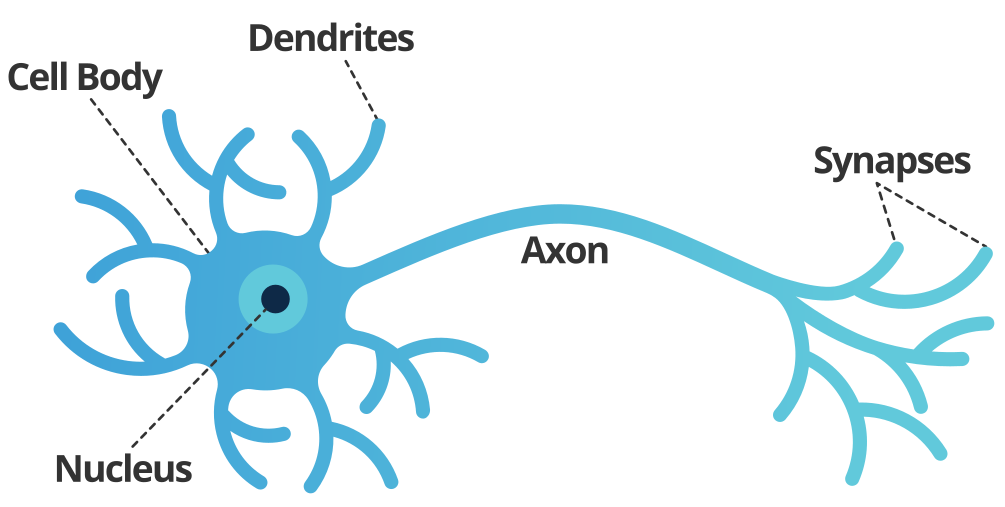
For a single neuron/node with input [math]u \in \mathbb{R}^{n}[/math], a mathematical model, named the perceptron [1], can be described as
where [math]y[/math] is the activation of the neuron/node, [math]W_i[/math] are the weights and [math]b[/math] is the bias.
The function [math]\sigma:\mathbb{R} \rightarrow \mathbb{R}[/math] is called activation function. Originally, in [1], it was proposed to choose the Heaviside function as activation function to model whether a neuron fires or not, i.e.
However, over time several other activation functions have been suggested and are being used. Typically, they are monotone increasing to remain in the spirit of the original idea, but continuous.
Popular activation functions are, cf. [2](p.90)
While the sigmoid function approximates the Heaviside function continuously, and is differentiable, it contains an exponential operation, which is computationally expensive. Similar problems arise with the hyperbolic tangent function. However, the fact that [math]\tanh[/math] is closer to the identity function often helps speed up convergence, since it resembles a linear model, as long as the values are close to zero. Another challenge that needs to be overcome is vanishing derivatives, which is visibly present for Heaviside, sigmoid and hyperbolic tangent. In contrast, ReLU is not bounded on positive values, while also being comparatively cheap to compute, because linear computations tend to be very well optimized in modern computing. Altogether, these advantages have resulted in ReLU (and variants thereof) becoming the most widely used activation function currently. As a remedy for the vanishing gradient on negative values, leaky ReLU was introduced. When taking derivatives of ReLU one needs to account for the non-differentiability at 0, but in numerical practice this is easily overcome.
With the help of Neural Networks we want to solve a task, cf. [3](Section 5.1). Let the performance of the algorithm for the given task be measured by the loss function [math]L[/math], which needs to be adequately modeled. By [math]\mathcal{F}[/math] we denote the Neural Network. The variables that will be learned are the weights [math]W[/math] and biases [math]b[/math] of the Neural Network. Hence, we can formulate the following optimization problem, cf. [4][5][6]
One possible choice for [math]\mathcal{F}[/math] has already been given in \eqref{eq:perceptron}, the perceptron. In the subsequent sections we introduce and analyze various other Neural Network architectures. They all have in common that they contain weights and biases, so that the above problem formulation remains sensible.
Before we move on to different network architectures, we discuss the modeling of the loss function. Learning tasks can be divided into two subgroups: Supervised and Unsupervised learning.
Supervised Learning
In supervised learning we have given data [math]u[/math] with known supervision [math]S(u)[/math] (also called labels), so that the task is to match the output [math]y[/math] of the Neural Network to the supervision. These problems are further categorized depending on the known supervision, e.g. for [math]S(u) \in \mathbb{N}[/math] it is called a classification and for [math]S(u) \in \mathbb{R}[/math] a regression. Furthermore, the supervision [math]S(u)[/math] can also take more complex forms like a black and white picture of [math]256 \times 256[/math] pixels represented by [math][0,1]^{256}[/math], a higher dimensional quantity, a sentence, etc. These cases are called structured output learning.
Let us consider one very simple example, cf. [3](Section 5.1.4).
Example
We have a given set of inputs [math]u^{(i)} \in \mathbb{R}^d[/math] with known supervisions [math]S(u^{(i)}) \in \mathbb{R}[/math] for [math]i=1,\ldots,N[/math]. In this example we only consider weights [math]W \in \mathbb{R}^{d}[/math] and no bias. Additionally, let [math]\sigma = \textrm{id}[/math]. The perceptron network simplifies to
and the learning task is to find [math]W[/math], such that [math]y^{(i)} \approx S(u^{(i)})[/math]. This can be modeled by the mean squared error (MSE) function
By convention we will use [math]\| \cdot \| = \| \cdot \|_2[/math] throughout the lecture. The chosen loss function is quadratic, convex and non-negative. We define
so that we can write [math]\mathscr{L}(W) = \frac{1}{2} \| U W - S\|_2^2 [/math]. Minimizing this function will deliver the same optimal weight [math]W[/math] as minimizing the MSE function defined above. We can now derive the gradient
and immediately find the stationary point [math]W = (U^{\top} U)^{-1} U^{\top} S[/math].
Unsupervised Learning
In unsupervised learning, only the input data [math]u[/math] is given and we have no knowledge of supervisions or labels. The algorithm is supposed to learn e.g. a structure or relation in the data. Some examples are k-clustering and principal component analysis (PCA). Modeling the loss function specifies the task and has a direct influence on the learning process. For illustration of this concept, we introduce the k-means algorithm, see eg. [2](Chapter 10), which is used for clustering.
Example
We have a set of given data points
and a desired number of clusters [math]k \in \mathbb{N}[/math] with [math]k \leq N[/math] and typically [math]k \ll N[/math]. Every data point is supposed to be assigned to a cluster.
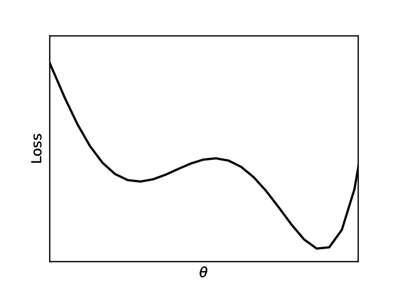
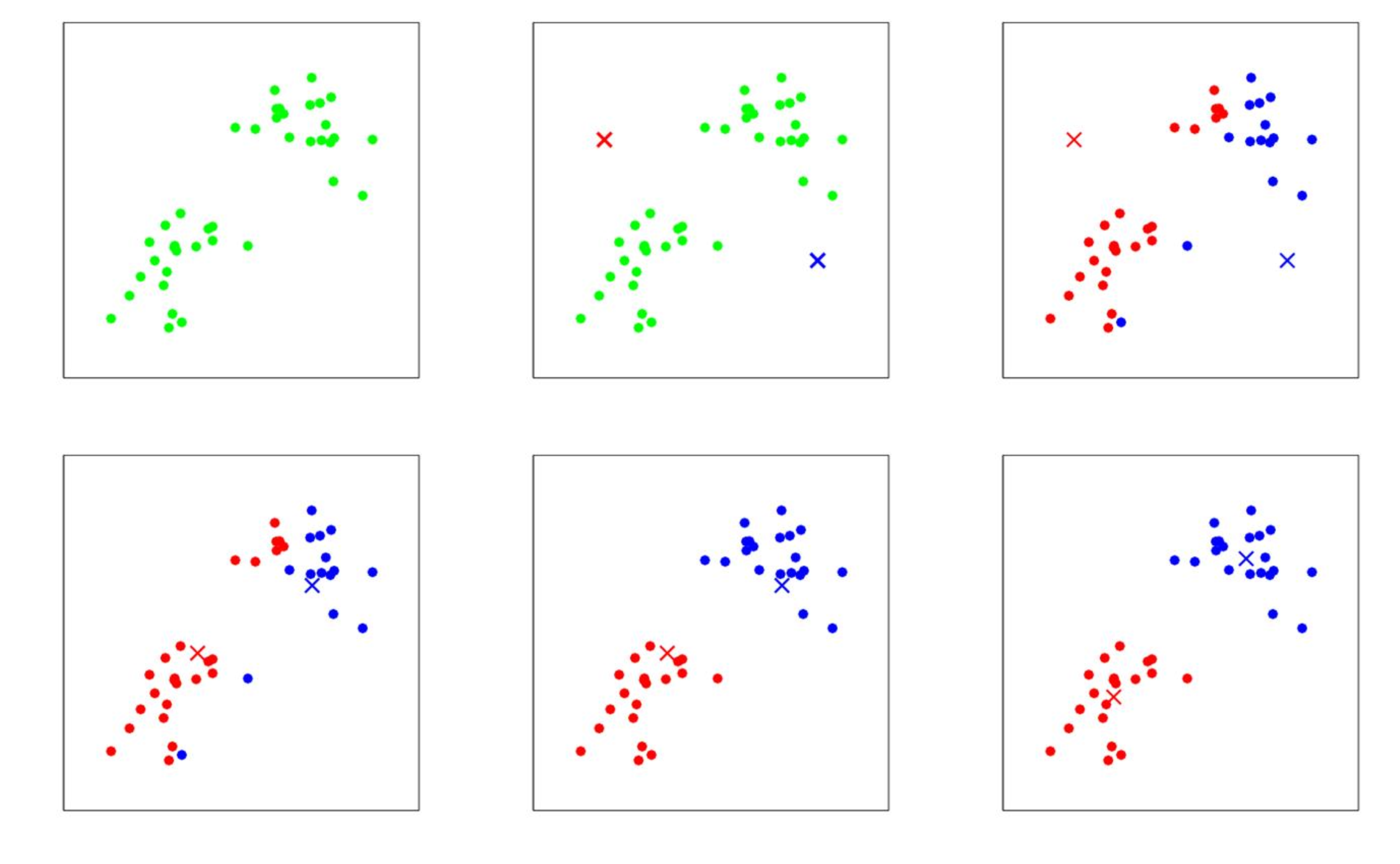
Iteratively every data point is assigned to the cluster with the nearest centroid, and we redefine cluster centroids as the mean of the vectors in the cluster. The procedure is specified in Algorithm k-means clustering and illustrated for an example in Figure, which can be found e.g. in [2](Chapter 10). The loss function (also called distortion function in this setup) can be defined as
which is also a model of the quantity that we try to minimize in Algorithm k-means clustering. We have a non-convex set of points in [math]\mathbb{R}^d[/math], so the algorithm may converge to a local minimum. To prevent this, we run the algorithm many times, compare the resulting clusterings using the loss function, and choose the one with the minimal value attained in the loss function.
Require: Initial cluster centroids [math]\mu_1,\ldots,\mu_k[/math]
We will see various other loss functions [math]\mathscr{L}[/math] throughout the remainder of this lecture, all of them specifically tailored to the task at hand.
In the case of Linear Regression, we have a closed form derivative, so we are able to find the solution by direct calculus, while for k-means clustering the optimization was done by a tailored iteration. For general problems we will need a suitable optimization algorithm. We move on to introduce a few options.
Optimization Algorithms
Here, for simplicity we define [math]\theta[/math], which collects all variables, i.e. weights [math]W[/math] and bias [math]b[/math] and write the loss function as
which we want to minimize. Here, [math]\mathscr{L}^{(i)}[/math] indicates the loss function evaluated for data point [math]i[/math], for example with a MSE loss [math]\mathscr{L}^{(i)}(\theta) = \frac{1}{2} \| y^{(i)} - S(u^{(i)}) \|^2[/math].
First, let us recall the standard gradient descent algorithm, see e.g. [7](Section 9.3), which is also known as steepest descent or batch gradient descent.
Require: Initial point [math]\theta^0[/math], step size [math]\tau\gt0[/math], counter [math]k=0[/math].
end while
Possible stopping criterion are e.g. setting a maximum number of iterations [math]k[/math], reaching a certain exactness [math]\|\mathscr{L}(\theta)\| \lt \epsilon [/math] with a small number [math]\epsilon\gt0[/math], or a decay in change [math]\| \theta^{k+1}-\theta^k\| \lt \epsilon[/math]. Determining a suitable step size is integral to the success of the gradient descent method, especially since this algorithm uses the same step size [math]\tau[/math] for all components of [math]\theta[/math], which can be a large vector in applications. If may happen that in some components the computed descent direction is only providing descent in a small neighborhood, therefore requiring a small step size [math]\tau[/math].
It is also possible to employ a line search algorithm. However, this is not common in Machine Learning currently. Instead, typically a small step size is chosen, so that it will (hopefully) be not too large for any component of [math]\theta[/math], and then it may be adaptively increased. Furthermore, let us remark that the step size is often called learning rate in a Machine Learning context.
Additionally, a grand challenge in Machine Learning tasks is that we have huge data sets, and the gradient descent algorithm has to iterate over all data points in every iteration, since [math]\mathscr{L}(\theta)[/math] contains all data points, which causes a tremendous computational cost. This motivates the use of the stochastic gradient descent algorithm, cf. [2](Algorithm 1), which only takes one data point into account per iteration.
Require: Initial point [math]\theta^0[/math], step size [math]\tau\gt0[/math], counter [math]k=0[/math], maximum number of iterations [math]K[/math].
Since the stochastic gradient descent method only calculates the gradient for one data point, it produces an irregular convergence behavior. Indeed, it does not necessarily converge at all, but for a large number of iterations [math]K[/math] it often produces a good approximation. In fact, actually converging in training the Neural Network is often not necessary/desired anyhow, since we want to have a solution that generalizes well to unseen data, rather than fit the given data points perfectly. Actually, the latter may lead to overfitting, cf. Section Overfitting and Underfitting.
Therefore, SGD is a computationally cheap, reasonable alternative to gradient descent.
As a compromise, which generates a less irregular convergence behavior, there also exists mini batch gradient descent, cf. [2](Algorithm 2), where every iteration takes into account a subset (mini batch) of the data points.
Require: Initial point [math]\theta^0[/math], step size [math]\tau\gt0[/math], counter [math]k=0[/math], maximum number of iterations [math]K[/math], batch size [math]b\in \mathbb{N}[/math].
end while
Finally, we introduce a sophisticated algorithm for stochastic optimization called Adam, [8], see Algorithm Adam. It is also a gradient-based method, and as an extension of the previous methods it employs adaptive estimates of so-called moments.
All operations on vectors are element-wise. [math](g^k)^2[/math] indicates the element-wise square [math]g^k \odot g^k[/math], and [math](\beta_1)^k, (\beta_2)^k[/math] denote the [math]k[/math]-th power of [math]\beta_1[/math] and [math]\beta_2[/math], respectively.
Require: Initial point [math]\theta^0[/math], step size [math]\tau\gt0[/math], counter [math]k=0[/math], exponential decay rates for the moment estimates [math]\beta_1,\beta_2 \in [0,1)[/math], [math]\epsilon \gt 0[/math], stochastic approximation [math]\widetilde{\mathscr{L}}(\theta)[/math] of the loss function.
end while
Good default settings in Adam for the tested machine learning problems are [math]\tau = 0.001[/math], [math]\beta_1 = 0.9, \beta_2 = 0.999[/math] and [math]\epsilon = 10^{-8}[/math], cf. [8]. Typically, the stochasticity of [math]\widetilde{\mathscr{L}}(\theta)[/math] will come from using mini batches of the data set, as in Mini Batch Gradient Descent, Algorithm Mini Batch Gradient Descent.
In the following section we discuss how fitting the given data points and generalizing well to unseen data can be contradictory goals.
Overfitting and Underfitting
As an example we discuss supervised learning with polynomials of degree [math]r[/math], cf. [9](Section 1.3.3). Example
Define
with [math]u=(u^0,...,u^r)^\top \in \mathbb{R}^{r+1}[/math] the potencies of data point [math]u[/math], and [math]W:=(W_0,...,W_r)^\top \in \mathbb{R}^{r+1}[/math]. The polynomial [math]p[/math] is linear in [math]W[/math], but not in [math]u[/math]. As in Linear Regression (Example), we do not consider bias [math]b[/math] here. Our goal is to compute weights [math]W[/math], given data points [math]u^{(i)}[/math] with supervisions [math]S(u^{(i)})[/math], so that [math]p[/math] makes good predictions on data it hasn't seen before. We again employ the MSE loss function
As before, we write the loss in matrix-vector notation
where
The minimizer [math]W[/math] can be directly calculated, cf. Example.
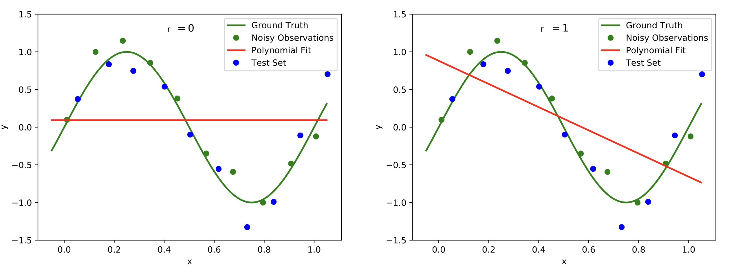
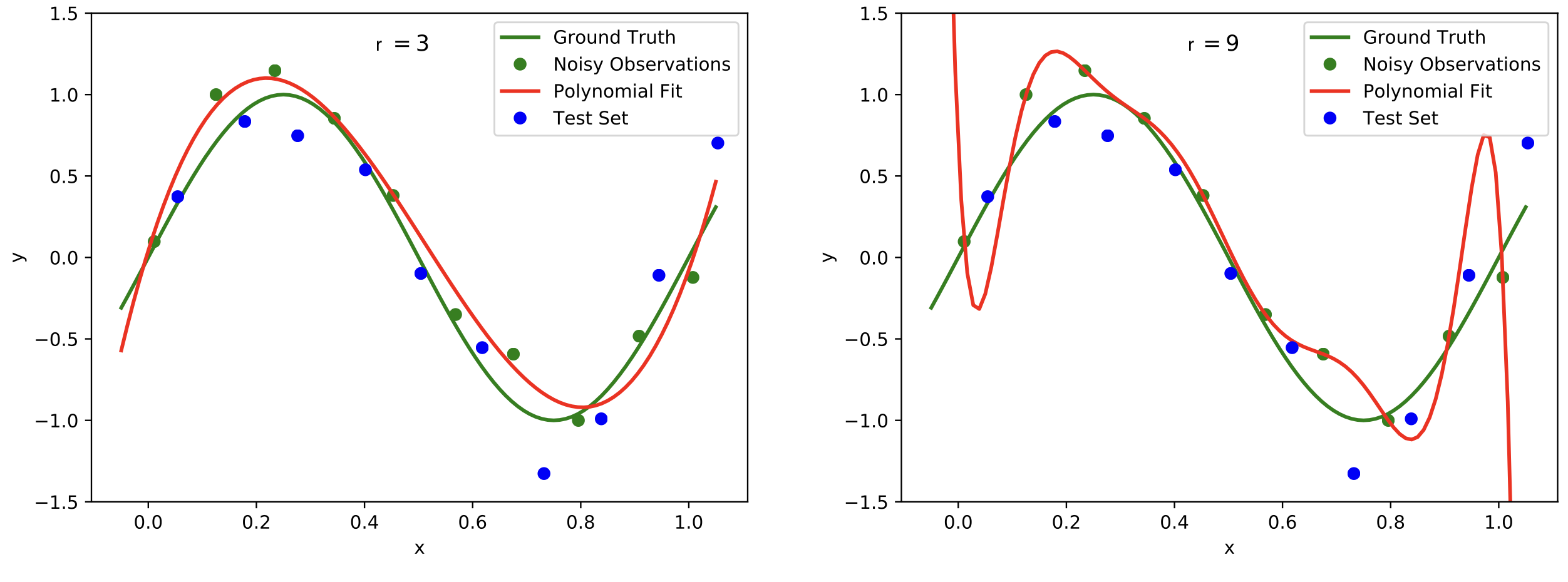
Plots of polynomials of various degrees r (red graph) fitted to the noisy data points (green dots) based on the ground truth (green graph). The model should extend well to the test set data (blue dots). We observe underfitting in the top row for [math]r=0[/math] (left) and [math]r=1[/math] (right). In the bottom left with [math]r=3[/math] reasonable results are achieved, while [math]r=9[/math] in the bottom right leads to overfitting. Image modified from: [9](Fig. 1).
To measure the performance of the polynomial curve fitting we compute the error on data points that were not used to determine the best polynomial fit, because we aim for a model that will generalize well. To this end, finding a suitable degree for the polynomial that we are fitting over the data points is crucial. If the degree is too low, we will encounter underfitting, see Figure top row. This means that the complexity of the polynomial is too low and the model does not even fit the data points. A remedy is to increase the degree of the polynomial, see Figure bottom left. However, increasing the degree too much may lead to overfitting, see Figure bottom right. The data points are fit perfectly, but the curve will not generalize well.
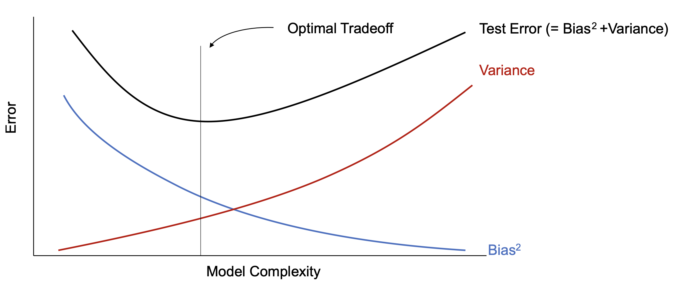
We can characterize overfitting and underfitting by using some statistics, cf. [2](Section 8.1). A point estimator [math]g:\mathcal{U}^N \rightarrow \Theta[/math] (where [math]\mathcal{U}[/math] denotes the data space, and [math]\Theta[/math] denotes the parameter space) is a function which makes an estimation of the underlying parameters of the model. For example, the estimate for [math]\theta=W[/math] from Example: [math]\hat{\theta}=(U^\top U)^{-1}U^\top S[/math] (which we will denote with a hat in this subsection to emphasize that it is an estimation) is an example of a point estimator. We assume that the data from [math]\mathcal{U}^N[/math] is i.i.d, so that [math]\hat{\theta}[/math] is a random variable. We can define the variance and the bias
with [math]\mathbb{E}[/math] denoting the expected value. A good estimator has both, low variance and low bias. We can characterize overfitting with low bias and high variance, and underfitting with high bias and low variance. The bias-variance trade-off is illustrated in Figure. Hence, we can make a decision based on mean squared error of the estimates
In general, it can be hard to guess a suitable degree for the polynomial beforehand. We could compute a fitting curve for different choices of [math]r[/math] and then compare the error on previously unseen data points of the validation data set, cf. Section Hyperparameters and Data Set Splitting , to determine which one generalizes best. This will require solving the problem multiple times which is unfavorable, especially for large data sets. Also, the polynomial degree can only be set discretely. Another, continuous way is to introduce a penalization term in the loss function
This technique is also called weight decay, cf. [3](Section 5.2.2). We can also use other norms, e.g. [math]\| \cdot \|_1[/math]. Here, we can choose a large degree [math]r[/math] and for [math]\lambda[/math] big enough, we will still avoid overfitting, because many components of [math]\theta[/math] will be (close to) zero. Nonetheless, we need to be cautious with the choice of [math]\lambda[/math]. If it is too big, we will face again the problem of underfitting.
We see that choosing values for the degree [math]r[/math] and the penalization parameter [math]\lambda[/math] poses challenges, and will discuss this further in the next section.
Hyperparameters and Data Set Splitting
We call all quantities that need to be chosen before solving the optimization problem hyperparameters, cf. [3](Section 5.3). Let us point out that hyperparameters are not learnt by the optimization algorithm itself, but nevertheless have an impact on the algorithms performance. Examples of hyperparameters include the polynomial degree [math]r[/math], the scalar [math]\lambda[/math], all parameters in the optimization algorithms (Section Optimization Algorithms ) like the step size [math]\tau[/math], and also the architecture of the Neural Network, and many more.
The impact of having a good set of hyperparameters can be tremendous, however finding such a set is not trivial. First of all, we split our given data into three sets. training data, validation data and test data (a 4:1:1 ratio is common). We have seen training and test data before. The data points that we are using as input to solve the optimization problem are called training data, and the unseen data points, which we use to evaluate whether the model generalizes well, are called test data. Since we don't want to mix different causes of error, we also introduce the validation data set. This will be used to compare different choices of hyperparameter configurations, i.e. we train the model on the training data for different hyperparameters, compute the error on the validation data set, choose the hyperparameter setup with the lowest error and finally evaluate the model on the test set. The reasoning behind this is that if we would use the test data set to determine the hyperparameter values, the test error may be not meaningful, because the hyperparameters have been optimized for this specific test set. Since we are using the validation set, we will have the test set with previously unseen data available to determine the generalization error without giving our network an advantage.
Still, imagine you need to choose 5 hyperparameters and have 4 possible values that you want to try for each hyperparameter. This amounts to [math]4^5 = 1024[/math] combinations you have to run on the training data and evaluate on the validation set. In real applications the number of hyperparameters and possible values can be much larger, so that it is nearly infeasible to try every combination, but rather common to change one hyperparameter at a time. Luckily, some hyperparameters also have known good default values, like the hyperparameters for Adam Optimizer, Algorithm Adam. Apart from that it is a tedious, manual work to try out, monitor and choose suitable hyperparameters.
Finally, we discuss the limitations of shallow Neural Networks, i.e. networks with only one layer.
Modeling logical functions
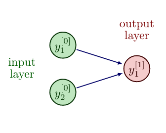
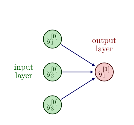
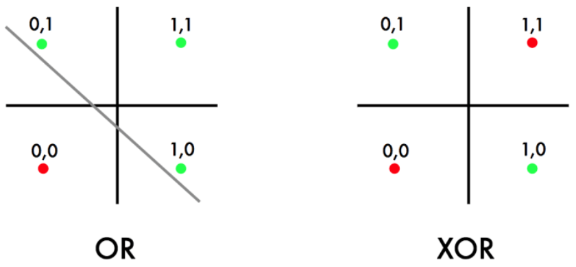
Let us consider a shallow Neural Network with input layer [math]y^{[0]} \in \mathbb{N}^2[/math] and output layer [math]y^{[1]} \in \mathbb{N}[/math].
We model true by the value 1 and false by the value 0, which results in the following truth table for the logical "OR" function.
| input [math]y^{[0]}_1[/math] | input [math]y^{[0]}_2[/math] | [math]y^{[0]}_1[/math] OR [math]y^{[0]}_2[/math] (output [math]y^{[1]}_1[/math]) |
| 0 | 0 | 0 |
| 1 | 0 | 1 |
| 0 | 1 | 1 |
| 1 | 1 | 1 |
With Heaviside activation function, we have
The goal is now to choose [math]W_1,W_2,b[/math] so that we match the output from the truth table for given input. Obviously, [math]W_1 = W_2 = 1[/math] and [math]b=-1[/math] is a possible choice that fulfills the task. Similarly, one can find values for [math]W_1,W_2[/math] and [math]b[/math] to model the logical "AND" function.
Next, let us consider the logical "XOR" function with the following truth table.
| input [math]y^{[0]}_1[/math] | input [math]y^{[0]}_2[/math] | [math]y^{[0]}_1[/math] XOR [math]y^{[0]}_2[/math] (output [math]y^{[1]}_1[/math]) |
| 0 | 0 | 0 |
| 1 | 0 | 1 |
| 0 | 1 | 1 |
| 1 | 1 | 0 |
In fact, the logical "XOR" function can not be represented by the given shallow Neural Network, since the data is not linearly separable, see e.g. [3](Section 6.1). This motivates the introduction of additional layers in between the input and output layer, i.e. we choose a more complex function [math]\mathcal{F}[/math] in the learning problem \eqref{eq:LP}.
General references
Herberg, Evelyn (2023). "Lecture Notes: Neural Network Architectures". arXiv:2304.05133 [cs.LG].
References
- 1.0 1.1 F. Rosenblatt. (1958). "The perceptron: a probabilistic model for information storage and organi- zation in the brain.". Psychological review 65. American Psychological Association.
- 2.0 2.1 2.2 2.3 2.4 2.5 2.6 2.7 2.8 Ng, A. (2022), CS229 Lecture Notes (PDF)
- 3.0 3.1 3.2 3.3 3.4 I. Goodfellow, Y. Bengio, and A. Courville. (2016). Deep learning. MIT Press.CS1 maint: multiple names: authors list (link)
- H. Antil, T. S. Brown, R. Löhner, F. Togashi, and D. Verma. (2022). "Deep Neural Nets with Fixed Bias Configuration". arXiv preprint arXiv:2107.01308.
- H. Antil and H. Díaz and E. Herberg (2022). "An Optimal Time Variable Learning Framework for Deep Neural Networks". arXiv preprint arXiv:2204.08528.
- H. Antil, R. Khatri, R. Löhner, and D. Verma. (2020). "Fractional deep neural network via constrained optimization". Machine Learning: Science and Technology 2. IOP Publishing.
- S. Boyd and L. Vandenberghe. (2004). Convex optimization. Cambridge university press.
- 8.0 8.1 Kingma, D. P. and Ba, J. (2014). "Adam: A method for stochastic optimization". arXiv preprint arXiv:1412.6980.
- 9.0 9.1 Geiger, A. (2021), Deep Learning Lecture Notes

