Three Components of ML
[math] % Generic syms \newcommand\defeq{:=} \newcommand{\Tt}[0]{\boldsymbol{\theta}} \newcommand{\XX}[0]{{\cal X}} \newcommand{\ZZ}[0]{{\cal Z}} \newcommand{\vx}[0]{{\bf x}} \newcommand{\vv}[0]{{\bf v}} \newcommand{\vu}[0]{{\bf u}} \newcommand{\vs}[0]{{\bf s}} \newcommand{\vm}[0]{{\bf m}} \newcommand{\vq}[0]{{\bf q}} \newcommand{\mX}[0]{{\bf X}} \newcommand{\mC}[0]{{\bf C}} \newcommand{\mA}[0]{{\bf A}} \newcommand{\mL}[0]{{\bf L}} \newcommand{\fscore}[0]{F_{1}} \newcommand{\sparsity}{s} \newcommand{\mW}[0]{{\bf W}} \newcommand{\mD}[0]{{\bf D}} \newcommand{\mZ}[0]{{\bf Z}} \newcommand{\vw}[0]{{\bf w}} \newcommand{\D}[0]{{\mathcal{D}}} \newcommand{\mP}{\mathbf{P}} \newcommand{\mQ}{\mathbf{Q}} \newcommand{\E}[0]{{\mathbb{E}}} \newcommand{\vy}[0]{{\bf y}} \newcommand{\va}[0]{{\bf a}} \newcommand{\vn}[0]{{\bf n}} \newcommand{\vb}[0]{{\bf b}} \newcommand{\vr}[0]{{\bf r}} \newcommand{\vz}[0]{{\bf z}} \newcommand{\N}[0]{{\mathcal{N}}} \newcommand{\vc}[0]{{\bf c}} % Statistics and Probability Theory \newcommand{\errprob}{p_{\rm err}} \newcommand{\prob}[1]{p({#1})} \newcommand{\pdf}[1]{p({#1})} \def \expect {\mathbb{E} } % Machine Learning Symbols \newcommand{\biasterm}{B} \newcommand{\varianceterm}{V} \newcommand{\neighbourhood}[1]{\mathcal{N}^{(#1)}} \newcommand{\nrfolds}{k} \newcommand{\mseesterr}{E_{\rm est}} \newcommand{\bootstrapidx}{b} %\newcommand{\modeldim}{r} \newcommand{\modelidx}{l} \newcommand{\nrbootstraps}{B} \newcommand{\sampleweight}[1]{q^{(#1)}} \newcommand{\nrcategories}{K} \newcommand{\splitratio}[0]{{\rho}} \newcommand{\norm}[1]{\Vert {#1} \Vert} \newcommand{\sqeuclnorm}[1]{\big\Vert {#1} \big\Vert^{2}_{2}} \newcommand{\bmx}[0]{\begin{bmatrix}} \newcommand{\emx}[0]{\end{bmatrix}} \newcommand{\T}[0]{\text{T}} \DeclareMathOperator*{\rank}{rank} %\newcommand\defeq{:=} \newcommand\eigvecS{\hat{\mathbf{u}}} \newcommand\eigvecCov{\mathbf{u}} \newcommand\eigvecCoventry{u} \newcommand{\featuredim}{n} \newcommand{\featurelenraw}{\featuredim'} \newcommand{\featurelen}{\featuredim} \newcommand{\samplingset}{\mathcal{M}} \newcommand{\samplesize}{m} \newcommand{\sampleidx}{i} \newcommand{\nractions}{A} \newcommand{\datapoint}{\vz} \newcommand{\actionidx}{a} \newcommand{\clusteridx}{c} \newcommand{\sizehypospace}{D} \newcommand{\nrcluster}{k} \newcommand{\nrseeds}{s} \newcommand{\featureidx}{j} \newcommand{\clustermean}{{\bm \mu}} \newcommand{\clustercov}{{\bm \Sigma}} \newcommand{\target}{y} \newcommand{\error}{E} \newcommand{\augidx}{b} \newcommand{\task}{\mathcal{T}} \newcommand{\nrtasks}{T} \newcommand{\taskidx}{t} \newcommand\truelabel{y} \newcommand{\polydegree}{r} \newcommand\labelvec{\vy} \newcommand\featurevec{\vx} \newcommand\feature{x} \newcommand\predictedlabel{\hat{y}} \newcommand\dataset{\mathcal{D}} \newcommand\trainset{\dataset^{(\rm train)}} \newcommand\valset{\dataset^{(\rm val)}} \newcommand\realcoorspace[1]{\mathbb{R}^{\text{#1}}} \newcommand\effdim[1]{d_{\rm eff} \left( #1 \right)} \newcommand{\inspace}{\mathcal{X}} \newcommand{\sigmoid}{\sigma} \newcommand{\outspace}{\mathcal{Y}} \newcommand{\hypospace}{\mathcal{H}} \newcommand{\emperror}{\widehat{L}} \newcommand\risk[1]{\expect \big \{ \loss{(\featurevec,\truelabel)}{#1} \big\}} \newcommand{\featurespace}{\mathcal{X}} \newcommand{\labelspace}{\mathcal{Y}} \newcommand{\rawfeaturevec}{\mathbf{z}} \newcommand{\rawfeature}{z} \newcommand{\condent}{H} \newcommand{\explanation}{e} \newcommand{\explainset}{\mathcal{E}} \newcommand{\user}{u} \newcommand{\actfun}{\sigma} \newcommand{\noisygrad}{g} \newcommand{\reconstrmap}{r} \newcommand{\predictor}{h} \newcommand{\eigval}[1]{\lambda_{#1}} \newcommand{\regparam}{\lambda} \newcommand{\lrate}{\alpha} \newcommand{\edges}{\mathcal{E}} \newcommand{\generror}{E} \DeclareMathOperator{\supp}{supp} %\newcommand{\loss}[3]{L({#1},{#2},{#3})} \newcommand{\loss}[2]{L\big({#1},{#2}\big)} \newcommand{\clusterspread}[2]{L^{2}_{\clusteridx}\big({#1},{#2}\big)} \newcommand{\determinant}[1]{{\rm det}({#1})} \DeclareMathOperator*{\argmax}{argmax} \DeclareMathOperator*{\argmin}{argmin} \newcommand{\itercntr}{r} \newcommand{\state}{s} \newcommand{\statespace}{\mathcal{S}} \newcommand{\timeidx}{t} \newcommand{\optpolicy}{\pi_{*}} \newcommand{\appoptpolicy}{\hat{\pi}} \newcommand{\dummyidx}{j} \newcommand{\gridsizex}{K} \newcommand{\gridsizey}{L} \newcommand{\localdataset}{\mathcal{X}} \newcommand{\reward}{r} \newcommand{\cumreward}{G} \newcommand{\return}{\cumreward} \newcommand{\action}{a} \newcommand\actionset{\mathcal{A}} \newcommand{\obstacles}{\mathcal{B}} \newcommand{\valuefunc}[1]{v_{#1}} \newcommand{\gridcell}[2]{\langle #1, #2 \rangle} \newcommand{\pair}[2]{\langle #1, #2 \rangle} \newcommand{\mdp}[5]{\langle #1, #2, #3, #4, #5 \rangle} \newcommand{\actionvalue}[1]{q_{#1}} \newcommand{\transition}{\mathcal{T}} \newcommand{\policy}{\pi} \newcommand{\charger}{c} \newcommand{\itervar}{k} \newcommand{\discount}{\gamma} \newcommand{\rumba}{Rumba} \newcommand{\actionnorth}{\rm N} \newcommand{\actionsouth}{\rm S} \newcommand{\actioneast}{\rm E} \newcommand{\actionwest}{\rm W} \newcommand{\chargingstations}{\mathcal{C}} \newcommand{\basisfunc}{\phi} \newcommand{\augparam}{B} \newcommand{\valerror}{E_{v}} \newcommand{\trainerror}{E_{t}} \newcommand{\foldidx}{b} \newcommand{\testset}{\dataset^{(\rm test)} } \newcommand{\testerror}{E^{(\rm test)}} \newcommand{\nrmodels}{M} \newcommand{\benchmarkerror}{E^{(\rm ref)}} \newcommand{\lossfun}{L} \newcommand{\datacluster}[1]{\mathcal{C}^{(#1)}} \newcommand{\cluster}{\mathcal{C}} \newcommand{\bayeshypothesis}{h^{*}} \newcommand{\featuremtx}{\mX} \newcommand{\weight}{w} \newcommand{\weights}{\vw} \newcommand{\regularizer}{\mathcal{R}} \newcommand{\decreg}[1]{\mathcal{R}_{#1}} \newcommand{\naturalnumbers}{\mathbb{N}} \newcommand{\featuremapvec}{{\bf \Phi}} \newcommand{\featuremap}{\phi} \newcommand{\batchsize}{B} \newcommand{\batch}{\mathcal{B}} \newcommand{\foldsize}{B} \newcommand{\nriter}{R} [/math]
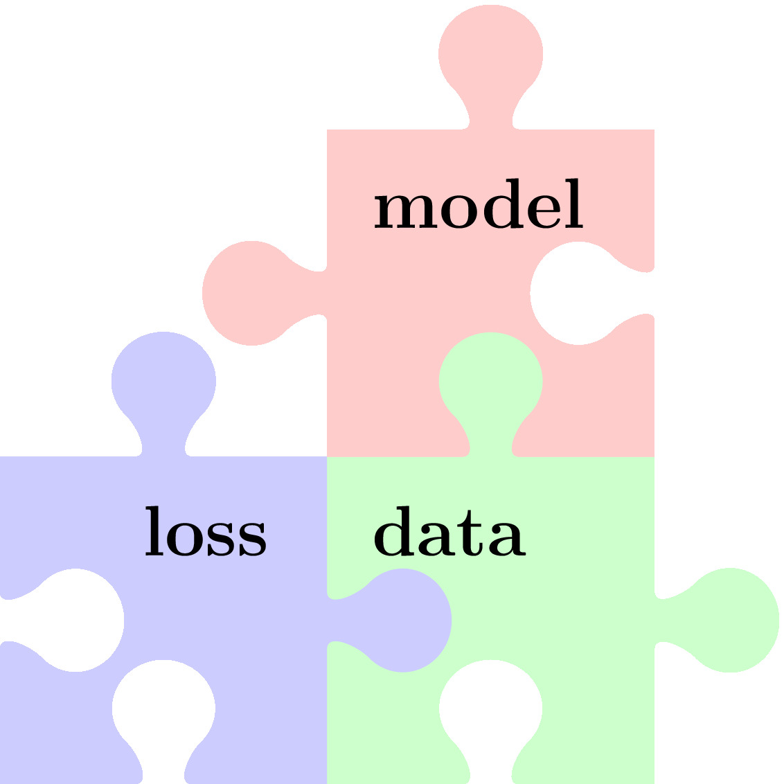
This book portrays ML as combinations of three components as depicted in Figure fig_ml_problem. These components are
- data as collections of individual data points that are characterized by features (see Section Features) and labels (see Section Labels)
- a model or hypothesis space that consists of computationally feasible hypothesis maps from feature space to label space (see Section The Model )
- a loss function (see Section The Loss ) to measure the quality of a hypothesis map.
A ML problem involves specific design choices for data points, its features and labels, the hypothesis space and the loss function to measure the quality of a particular hypothesis. Similar to ML problems (or applications), we can also characterize ML methods as combinations of these three components. This chapter discusses in some depth each of the above ML components and their combination within some widely-used ML methods [1].
We detail in Chapter The Landscape of ML how some of the most popular ML methods, including linear regression (see Section Linear Regression ) as well as deep learning methods (see Section Deep Learning ), are obtained by specific design choices for the three components. Chapter Empirical Risk Minimization will then introduce ERM as a main principle for how to operationally combine the individual ML components. Within the ERM principle, ML problems become optimization problems and ML methods become optimization methods.
The Data
Data as Collections of Data points. Maybe the most important component of any ML problem (and method) is data. We consider data as collections of individual data points which are atomic units of “information containers”. Data points can represent text documents, signal samples of time series generated by sensors, entire time series generated by collections of sensors, frames within a single video, random variables, videos within a movie database, cows within a herd, trees within a forest, or forests within a collection of forests. Mountain hikers might be interested in data points that represent different hiking tours (see Figure fig:image).
We use the concept of data points in a very abstract and therefore highly flexible manner. Data points can represent very different types of objects that arise in fundamentally different application domains. For an image processing application it might be useful to define data points as images. When developing a recommendation system we might define data points to represent customers. In the development of new drugs we might use data points to represent different diseases. Ultimately, the choice or definition of data points is a design choice. We might refer to the task of finding a useful definition of data points as “data point engineering”.
One practical requirement for a useful definition of data points is that we should have access to many of them. Many ML methods construct estimates for a quantity of interest (such as a prediction or forecast) by averaging over a set of reference (or training) data points. These estimates become more accurate for an increasing number of data points used for computing the average.
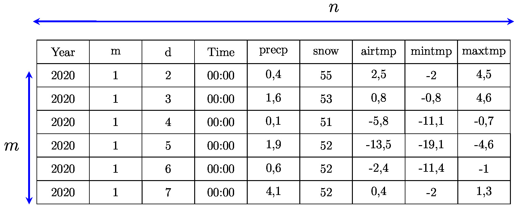
A key property of a dataset is the number [math]\samplesize[/math] of individual data points it contains. The number of data points within a dataset is also referred to as the sample size. From a statistical point of view, the larger the sample size [math]\samplesize[/math] the better. However, there might be restrictions on computational resources (such as memory size) that limit the maximum sample size [math]\samplesize[/math] that can be processed.
For most applications, it is impossible to have full access to every single microscopic property of a data point. Consider a data point that represents a vaccine. A full characterization of such a data point would require to specify its chemical composition down to level of molecules and atoms. Moreover, there are properties of a vaccine that depend on the patient who received the vaccine.
We find it useful to distinguish between two different groups of properties of a data point. The first group of properties is referred to as features and the second group of properties is referred to as labels. Roughly speaking, features are low-level properties of a data point that can be measured or computed easily in an automated fashion. In contract, labels are high-level properties of a data points that represent some quantity of interest. Determining the label value of a data point often requires human labour, e.g., a domain expert who has to examine the data point. Some widely used synonyms for features are “covariate”,“explanatory variable”, “independent variable”, “input (variable)”, “predictor (variable)” or “regressor” [2][3][4]. Some widely used synonyms for the label of a data point are "response variable", "output variable" or "target" [2][3][4].
We will discuss the concepts of features and labels in somewhat more detail in Sections Features and Labels. However, we would like to point out that the distinction between features and labels is blurry. The same property of a data point might be used as a feature in one application, while it might be used as a label in another application. Let us illustrate this blurry distinction between features and labels using the problem of missing data.
Assume we have a list of data points each of which is characterized by several properties that could be measured easily in principles (by sensors). These properties would be first candidates for being used as features of the data points. However, some of these properties are unknown (missing) for a small set of data points (e.g., due to broken sensors). We could then define the properties which are missing for some data points as labels and try to predict these labels using the remaining properties (which are known for all data points) as features. The task of determining missing values of properties that could be measured easily in principle is referred to as imputation [5].
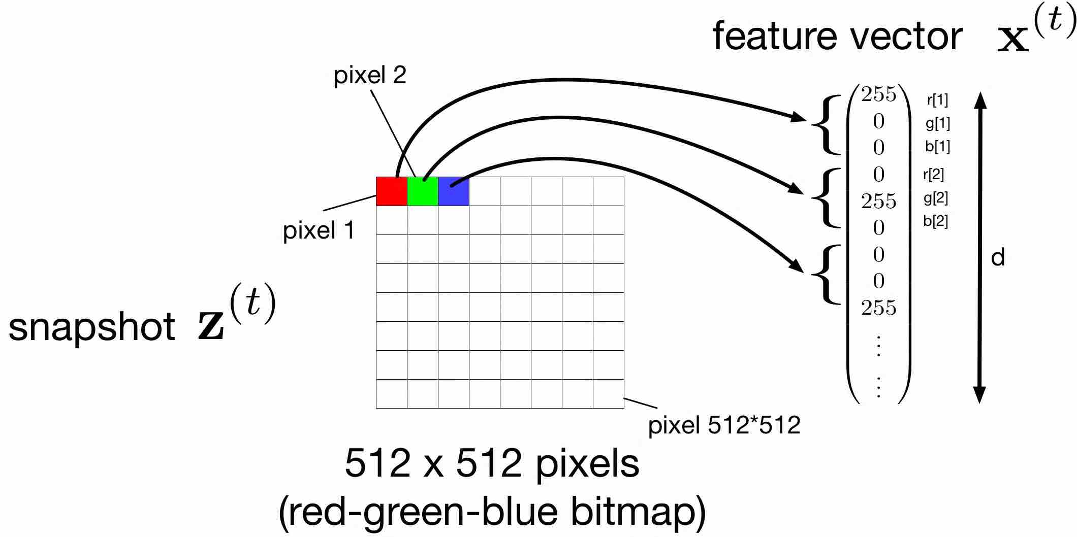
Missing data might also arise in image processing applications. Consider data points being images (snapshots) generated by a smartphone camera. Maybe the most intuitive choice for the features of a (bitmap) image are the colour intensities for each pixel (see Figure fig_snapshot_pixels). Due to hardware failures some of the image pixels might be corrupted or (their colour intensities) even completely missing. We could then try to use to learn to predict the colour intensities of a pixel based on the colour intensities of the neighbouring pixels. To this end, we might define new data points as small rectangular regions (patches) of the image and use the colour intensity of the centre pixel (“target pixel”) as the label of such a patch.
Figure fig:two_main_parameters illustrates two key properties of a dataset. The first property is the sample size [math]\samplesize[/math], i.e., the number of individual data points that constitute the dataset. The second key property of is the number [math]\featurelen[/math] of features that are used to characterize an individual data point. The behaviour of ML methods often depends crucially on the ratio [math]\samplesize/\featurelen[/math]. The performance of ML methods typically improves with increasing [math]\samplesize/\featurelen[/math]. As a rule of thumb, we should use datasets for which [math]\samplesize/\featurelen \gg 1[/math]. We will make the informal condition [math]\samplesize / \featurelen \gg 1[/math] more precise in Chapter Model Validation and Selection .
Features
Similar to the choice (or definition) of data points with an ML application, also the choice of which properties to be used as their features is a design choice. In general, features are (low-level) properties of a data point that can be computed or measured easily. This is obviously a highly informal characterization since there is no universal criterion for the difficulty of computing of measuring a specific property of data points. The task of choosing which properties to use as features of data points might be the most challenging part in the application of ML methods. Chapter Feature Learning discusses feature learning methods that automate (to some extend) the construction of good features.
In some application domains there is a rather natural choice for the features of a data point. For data points representing audio recording (of a given duration) we might use the signal amplitudes at regular sampling instants (e.g., using sampling frequency [math]44[/math] kHz) as features. For data points representing images it seems natural to use the colour (red, green and blue) intensity levels of each pixel as a feature (see Figure fig_snapshot_pixels).
The feature construction for images depicted in Figure fig_snapshot_pixels can be extended to other types of data points as long as they can be visualized efficiently [6]. Audio recordings are typically available a sequence of signal amplitudes [math]a_{\timeidx}[/math] collected regularly at time instants [math]\timeidx=1,\ldots,\featuredim[/math] with sampling frequency [math]\approx 44[/math] kHz. From a signal processing perspective, it seems natural to directly use the signal amplitudes as features, [math]\feature_{\featureidx} = a_{\featureidx}[/math] for [math]\featureidx=1,\ldots,\featurelen[/math]. However, another choice for the features would be the pixel RGB values of some visualization of the audio recording.
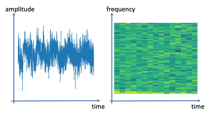
Figure fig_visualization_audio depicts two possible visualizations of an audio signal. The first visualization is obtained from a line plot of the signal amplitudes as a function of time [math]\timeidx[/math]. Another visualization of an audio recording is obtained from an intensity plot of its spectrogram[7][8]. We can then use the pixel RGB intensities of these visualizations as the features for an audio recording. Using this trick we can transform any ML method for image data to an ML method for audio data. We can use the scatterplot of a data set to use ML methods for image segmentation to cluster the dataset(see Chapter Clustering ).
Many important ML application domains generate data points that are characterized by several numeric features [math]x_{1},\ldots,x_{\featuredim}[/math]. We represent numeric features by real numbers [math]x_{1},\ldots,x_{\featuredim} \in \mathbb{R}[/math] which might seem impractical. Indeed, digital computers cannot store a real number exactly as this would require an infinite number of bits. However, numeric linear algebra soft- and hardware allows to approximate real numbers with sufficient accuracy. The majority of ML methods discussed in this book assume that data points are characterized by real-valued features. Section Feature Learning for Non-Numeric Data discusses methods for constructing numeric features of data points whose natural representation is non-numeric.
We assume that data points arising in a given ML application are characterized by the same number [math]\featurelen[/math] of individual features [math]\feature_{1}.\ldots,\feature_{\featurelen}[/math]. It is convenient to stack the individual features of a data point into a single feature vector
Each data point is then characterized by its feature vector [math]\featurevec[/math]. Note that stacking the features of a data point into a column vector [math]\featurevec[/math] is pure convention. We could also arrange the features as a row vector or even as a matrix, which might be even more natural for features obtained by the pixels of an image (see Figure fig_snapshot_pixels).
We refer to the set of possible feature vectors of data points arising in some ML application as the feature space and denote it as [math]\featurespace[/math]. The feature space is a design choice as it depends on what properties of a data point we use as its features. This design choice should take into account the statistical properties of the data as well as the available computational infrastructure. If the computational infrastructure allows for efficient numerical linear algebra, then using [math]\featurespace = \mathbb{R}^{\featurelen}[/math] might be a good choice.
The Euclidean space [math]\mathbb{R}^{\featuredim}[/math] is an example of a feature space with a rich geometric and algebraic structure [9]. The algebraic structure of [math]\mathbb{R}^{\featuredim}[/math] is defined by vector addition and multiplication of vectors with scalars. The geometric structure of [math]\mathbb{R}^{\featuredim}[/math] is obtained by the Euclidean norm as a measure for the distance between two elements of [math]\mathbb{R}^{\featuredim}[/math]. The algebraic and geometric structure of [math]\mathbb{R}^{\featuredim}[/math] often enables an efficient search over [math]\mathbb{R}^{\featuredim}[/math] to find elements with desired properties. Chapter ERM for Linear Regression discusses examples of such search problems in the context of learning an optimal hypothesis.
Modern information-technology, including smartphones or wearables, allows us to measure a huge number of properties about data points in many application domains. Consider a data point representing the book author “Alex Jung”. Alex uses a smartphone to take roughly five snapshots per day (sometimes more, e.g., during a mountain hike) resulting in more than [math]1000[/math] snapshots per year. Each snapshot contains around [math]10^{6}[/math] pixels whose greyscale levels we can use as features of the data point. This results in more than [math]10^{9}[/math] features (per year!).
As indicated above, many important ML applications involve data points represented by very long feature vectors. To process such high-dimensional data, modern ML methods rely on concepts from high-dimensional statistics [10][11]. One such concept from high-dimensional statistics is the notion of sparsity. Section The Lasso discusses methods that exploit the tendency of high-dimensional data points, which are characterized by a large number [math]\featuredim[/math] of features, to concentrate near low-dimensional subspaces in the feature space [12].
At first sight it might seem that “the more features the better” since using more features might convey more relevant information to achieve the overall goal. However, as we discuss in Chapter Regularization , it can be detrimental for the performance of ML methods to use an excessive amount of (irrelevant) features. Computationally, using too many features might result in prohibitive computational resource requirements (such as processing time). Statistically, each additional feature typically introduces an additional amount of noise (due to measurement or modelling errors) which is harmful for the accuracy of the ML method.
It is difficult to give a precise and broadly applicable characterization of the maximum number of features that should be used to characterize the data points. As a rule of thumb, the number [math]\samplesize[/math] of (labeled) data points used to train a ML method should be much larger than the number [math]\featurelen[/math] of numeric features (see Figure fig:two_main_parameters). The informal condition [math]\samplesize/\featurelen \gg 1[/math] can be ensured by either collecting a sufficiently large number [math]\samplesize[/math] of data points or by using a sufficiently small number [math]\featurelen[/math] of features. We next discuss implementations for each of these two complementary approaches.
The acquisition of (labeled) data points might be costly, requiring human expert labour. Instead of collecting more raw data, it might be more efficient to generate new artificial (synthetic) data via data augmentation techniques. Section Data Augmentation shows how intrinsic symmetries in the data can be used to augment the raw data with synthetic data. As an example for an intrinsic symmetry of data, consider data points being images. We assign each image the label [math]\truelabel=1[/math] if it shows a cat and [math]\truelabel=-1[/math] otherwise. For each image with known label we can generate several augmented (additional) images with the same label. These additional images might be obtained by simple image transformation such as rotations or re-scaling (zoom-in or zoom-out) that do not change the depicted objects (the meaning of the image). Chapter Regularization shows that some basic regularization techniques can be interpreted as an implicit form of data augmentation.
The informal condition [math]\samplesize/\featurelen \gg 1[/math] can also be ensured by reducing the number [math]\featurelen[/math] of features used to characterize data points. In some applications, we might use some domain knowledge to choose the most relevant features. For other applications, it might be difficult to tell which quantities are the best choice for features. Chapter Feature Learning discusses methods that learn, based on some given dataset, to determine a small number of relevant features of data points.
Beside the available computational infrastructure, also the statistical properties of datasets must be taken into account for the choices of the feature space. The linear algebraic structure of [math]\mathbb{R}^{\featuredim}[/math] allows us to efficiently represent and approximate datasets that are well aligned along linear subspaces. Section Principal Component Analysis discusses a basic method to optimally approximate datasets by linear subspaces of a given dimension. The geometric structure of [math]\mathbb{R}^{\featuredim}[/math] is also used in Chapter Clustering to decompose a dataset into few groups or clusters that consist of similar data points.
Throughout this book we will mainly use the feature space [math]\mathbb{R}^{\featuredim}[/math] with dimension [math]\featuredim[/math] being the number of features of a data point. This feature space has proven useful in many ML applications due to availability of efficient soft- and hardware for numerical linear algebra. Moreover, the algebraic and geometric structure of [math]\mathbb{R}^{\featuredim}[/math] reflect the intrinsic structure of data arising in many important application domains. This should not be too surprising as the Euclidean space has evolved as a useful mathematical abstraction of physical phenomena [13].
In general there is no mathematically correct choice for which properties of a data point to be used as its features. Most application domains allow for some design freedom in the choice of features. Let us illustrate this design freedom with a personalized health-care applications. This application involves data points that represent audio recordings with the fixed duration of three seconds. These recordings are obtained via smartphone microphones and used to detect coughing [14].
Labels
Besides its features, a data point might have a different kind of properties. These properties represent a higher-level fact or quantity of interest that is associated with the data point. We refer to such properties of a data point as its label (or “output” or “target”) and typically denote it by [math]\truelabel[/math] (if it is a single number) or by [math]\mathbf{\truelabel}[/math] (if it is a vector of different label values, such as in multi-label classification). We refer to the set of all possible label values of data points arising in a ML application is the label space [math]\labelspace[/math]. In general, determining the label of a data point is more difficult (to automate) compared to determining its features. Many ML methods revolve around finding efficient ways to predict (estimate or approximate) the label of a data point based solely on its features.
The distinction of data point properties into labels and features is blurry. Roughly speaking, labels are properties of data points that might only be determined with the help of human experts. For data points representing humans we could define its label [math]\truelabel[/math] as an indicator if the person has flu ([math]\truelabel=1[/math]) or not ([math]\truelabel=0[/math]). This label value can typically only be determined by a physician. However, in another application we might have enough resources to determine the flu status of any person of interest and could use it as a feature that characterizes a person.
Consider a data point that represents a hike, at the start of which the snapshot in Figure fig:image has been taken. The features of this data point could be the red, green and blue (RGB) intensities of each pixel in the snapshot in Figure fig:image. We stack these RGB values into a vector [math]\featurevec \in \mathbb{R}^{\featurelen}[/math] whose length [math]\featurelen[/math] is three times the number of pixels in the image. The label [math]\truelabel[/math] associated with a data point (a hike) could be the expected hiking time to reach the mountain in the snapshot. Alternatively, we could define the label [math]\truelabel[/math] as the water temperature of the lake that is depicted in the snapshot.
Numeric Labels - Regression.
For a given ML application, the label space [math]\labelspace[/math] contains all possible label values of data points. In general, the label space is not just a set of different elements but also equipped (algebraic or geometric) structure. To obtain efficient ML methods, we should exploit such structure. Maybe the most prominent example for such a structured label space are the real numbers [math]\labelspace = \mathbb{R}[/math]. This label space is useful for ML applications involving data points with numeric labels that can be modelled by real numbers. ML methods that aim at predicting a numeric label are referred to as regression methods.
Categorical Labels - Classification. Many important ML applications involve data points whose label indicate the category or class to which data points belongs to. ML methods that aim at predicting such categorical labels are referred to as classification methods. Examples for classification problems include the diagnosis of tumours as benign or maleficent, the classification of persons into age groups or detecting the current floor conditions ( “grass”, “tiles” or “soil”) for a mower robot.
The most simple type of a classification problems is a binary classification problem. Within binary classification, each data point belongs to exactly one out of two different classes. Thus, the label of a data point takes on values from a set that contains two different elements such as [math]\{0,1\}[/math] or [math]\{-1,1\}[/math] or [math]\{\mbox{“shows cat”}, \mbox{“shows no cat”}\}[/math].
We speak of a multi-class classification problem if data points belong to exactly one out of more than two categories (e.g., image categories “no cat shown” vs. “one cat shown” and “more than one cat shown”). If there are [math]\nrcategories[/math] different categories we might use the label values [math]\{1,2,\ldots, \nrcategories\}[/math].
There are also applications where data points can belong to several categories simultaneously. For example, an image can be cat image and a dog image at the same time if it contains a dog and a cat. Multi-label classification problems and methods use several labels [math]\truelabel_{1},\truelabel_{2},\ldots,[/math] for different categories to which a data point can belong to. The label [math]\truelabel_{\featureidx}[/math] represents the [math]\featureidx[/math]th category and its value is [math]\truelabel_{\featureidx}=1[/math] if the data point belongs to the [math]\featureidx[/math]-th category and [math]\truelabel_{\featureidx}=0[/math] if not.
Ordinal Labels. Ordinal label values are somewhat in between numeric and categorical labels. Similar to categorical labels, ordinal labels take on values from a finite set. Moreover, similar to numeric labels, ordinal labels take on values from an ordered set. For an example for such an ordered label space, consider data points representing rectangular areas of size [math]1[/math] km by [math]1[/math] km. The features [math]\featurevec[/math] of such a data point can be obtained by stacking the RGB pixel values of a satellite image depicting that area (see Figure fig_snapshot_pixels). Beside the feature vector, each rectangular area is characterized by a label [math]\truelabel \in \{1,2,3\}[/math] where
- [math]\truelabel=1[/math] means that the area contains no trees.
- [math]\truelabel=2[/math] means that the area is partially covered by trees.
- [math]\truelabel=3[/math] means that the are is entirely covered by trees.
Thus we might say that label value [math]\truelabel=2[/math] is “larger” than label value [math]\truelabel=1[/math] and label value [math]\truelabel=3[/math] is “larger” than label value [math]\truelabel=2[/math].
The distinction between regression and classification problems and methods is somewhat blurry. Consider a binary classification problem based on data points whose label [math]\truelabel[/math] takes on values [math]-1[/math] or [math]1[/math]. We could turn this into a regression problem by using a new label [math]\truelabel'[/math] which is defined as the confidence in the label [math]\truelabel[/math] being equal to [math]1[/math]. On the other hand, given a prediction [math]\hat{\truelabel'}[/math] for the numeric label [math]\truelabel' \in \mathbb{R}[/math] we can obtain a prediction [math]\hat{\truelabel}[/math] for the binary label [math]\truelabel \in \{-1,1\}[/math] by setting [math]\hat{\truelabel} \defeq 1[/math] if [math]\hat{\truelabel'} \geq0[/math] and [math]\hat{\truelabel}\defeq-1[/math] otherwise. A prominent example for this link between regression and classification is logistic regression which is discussed in Section Logistic Regression . Logistic regression is a binary classification method that uses the same model as linear regression but a different loss function.
We refer to a data point as being \emph{labeled} if, besides its features [math]\featurevec[/math], the value of its label [math]\truelabel[/math] is known. The acquisition of labeled data points typically involves human labour, such as verifying if an image shows a cat. In other applications, acquiring labels might require sending out a team of marine biologists to the Baltic sea [15], to run a particle physics experiment at the European organization for nuclear research (CERN) [16], or to conduct animal trials in pharmacology [17].
Let us also point out online market places for human labelling workforce [18]. These market places, allow to upload data points, such as collections of images or audio recordings, and then offer an hourly rate to humans that label the data points. This labeling work might amount to marking images that show a cat.
Many applications involve data points whose features can be determined easily, but whose labels are known for few data points only. Labeled data is a scarce resource. Some of the most successful ML methods have been devised in application domains where label information can be acquired easily [19]. ML methods for speech recognition and machine translation can make use of massive labeled datasets that are freely available [20].
In the extreme case, we do not know the label of any single data point. Even in the absence of any labeled data, ML methods can be useful for extracting relevant information from features only. We refer to ML methods which do not require any labeled data points as “unsupervised” ML methods. We discuss some of the most important unsupervised ML methods in Chapter Clustering and Chapter Feature Learning ).
ML methods learn (or search for) a “good” predictor [math]h: \featurespace \rightarrow \labelspace[/math] which takes the features [math]\featurevec \in \featurespace[/math] of a data point as its input and outputs a predicted label (or output, or target) [math]\hat{\truelabel} = h(\featurevec) \in \labelspace[/math]. A good predictor should be such that [math]\hat{\truelabel} \approx \truelabel[/math], i.e., the predicted label [math]\hat{\truelabel}[/math] is close (with small error [math]\hat{\truelabel} - \truelabel[/math]) to the true underlying label [math]\truelabel[/math].
Scatterplot
Consider data points characterized by a single numeric feature [math]\feature[/math] and single numeric label [math]\truelabel[/math]. To gain more insight into the relation between the features and label of a data point, it can be instructive to generate a scatterplot as shown in Figure fig_scatterplot_temp_FMI. A scatterplot depicts the data points [math]\datapoint^{(\sampleidx)}=(\feature^{(\sampleidx)},\truelabel^{(\sampleidx)})[/math] in a two-dimensional plane with the axes representing the values of feature [math]\feature[/math] and label [math]\truelabel[/math].
The visual inspection of a scatterplot might suggest potential relationships between feature [math]\feature[/math] (minimum daytime temperature) and label [math]\truelabel[/math] (maximum daytime temperature). From Figure fig_scatterplot_temp_FMI, it seems that there might be a relation between feature [math]\feature[/math] and label [math]\truelabel[/math] since data points with larger [math]\feature[/math] tend to have larger [math]\truelabel[/math]. This makes sense since having a larger minimum daytime temperature typically implies also a larger maximum daytime temperature.
To construct a scatterplot for data points with more than two features we can use feature learning methods (see Chapter Feature Learning ). These methods transform high-dimensional data points, having billions of raw features, to three or two new features. These new features can then be used as the coordinates of the data points in a scatterplot.
Probabilistic Models for Data
A powerful idea in ML is to interpret each data points as the realization of a random variable (RV). For ease of exposition let us consider data points that are characterized by a single feature [math]\feature[/math]. The following concepts can be extended easily to data points characterized by a feature vector [math]\featurevec[/math] and a label [math]\truelabel[/math].
One of the most basic examples of a probabilistic model for data points in ML is the independent and identically distributed (iid) assumption. This assumption interprets data points [math]\feature^{(1)},\ldots,\feature^{(\samplesize)}[/math] as realizations of statistically independent RVs with the same probability distribution [math]p(\feature)[/math]. It might not be immediately clear why it is a good idea to interpret data points as realizations of RVs with the common probability distribution [math]p(\feature)[/math]. However, this interpretation allows us to use the properties of the probability distribution to characterize overall properties of entire datasets, i.e., large collections of data points.
The probability distribution [math]p(\feature)[/math] underlying the data points within the i.i.d. assumption is either known (based on some domain expertise) or estimated from data. It is often enough to estimate only some parameters of the distribution [math]p(\feature)[/math]. Section Maximum Likelihood discusses a principled approach to estimate the parameters of a probability distribution from a given set of data points. This approach is sometimes referred to as maximum likelihood and aims at finding (parameter of) a probability distribution [math]p(\feature)[/math] such that the probability (density) of observing the given data points is maximized [21][22][23].
Two of the most basic and widely used parameters of a probability distribution [math]p(\feature)[/math] are the expected value or mean [24] [math]\mu_{\feature} = \expect\{\feature\} \defeq \int_{\feature'} \feature' p(\feature') dx'[/math] and the variance [math]\sigma_{\feature}^{2} \defeq \expect\big\{\big(\feature-\expect\{\feature\}\big)^{2}\big\}.[/math] These parameters can be estimated using the sample mean (average) and sample variance,
The sample mean and sample variance \eqref{equ_sample_mean_var} are the maximum likelihood estimators for the mean and variance of a normal (Gaussian) distribution [math]p(\feature)[/math] (see [25](Chapter 2.3.4)).
Most of the ML methods discussed in this book are motivated by an i.i.d. assumption. It is important to note that this i.i.d. assumption is only a modelling assumption (or hypothesis). There is no means to verify if an arbitrary set of data points are “exactly” realizations of iid RVs. There are principled statistical methods (hypothesis tests) that allow to verify if a given set of data point can be well approximated as realizations of iid RVs [26]. Alternatively, we can enforce the i.i.d. assumption if we generate synthetic data using a random number generator. Such synthetic iid data points could be obtained by sampling algorithms that incrementally build a synthetic dataset by adding randomly chosen raw data points [27].
The Model
Consider some ML application that generates data points, each characterized by features [math]\featurevec \in \featurespace[/math] and label [math]\truelabel \in \labelspace[/math]. The goal of a ML method is to learn a hypothesis map [math]h: \featurespace \rightarrow \labelspace[/math] such that
The informal goal \eqref{equ_approx_label_pred} will be made precise in several aspects throughout the rest of our book. First, we need to quantify the approximation error \eqref{equ_approx_label_pred} incurred by a given hypothesis map [math]h[/math]. Second, we need to make precise what we actually mean by requiring \eqref{equ_approx_label_pred} to hold for “any” data point. We solve the first issue by the concept of a loss function in Section The Loss . The second issue is then solved in Chapter Empirical Risk Minimization by using a simple probabilistic model for data.
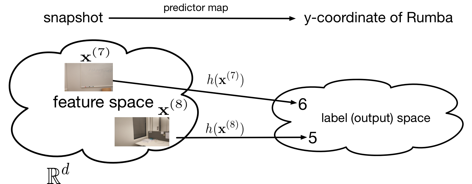
Let us assume for the time being that we have found a reasonable hypothesis [math]h[/math] in the sense of \eqref{equ_approx_label_pred}. We can then use this hypothesis to predict the label of any data point for which we know its features. The prediction [math]\hat{\truelabel}=h(\featurevec)[/math] is obtained by evaluating the hypothesis for the features [math]\featurevec[/math] of a data point (see Figure fig_feature_map_eval and fig:Hypothesis_Map). We refer to a hypothesis map also as a predictor map since it is used or compute the prediction [math]\hat{\truelabel}[/math] of a (true) label [math]\truelabel[/math].
For ML problems using a finite label space [math]\labelspace[/math] (e..g, [math]\labelspace=\{-1,1\}[/math], we refer to a hypothesis also as a classifier. For a finite \label{labelspace} [math]\labelspace[/math], we can characterize a particular classifier map [math]h[/math] using its different decision regions
Each label value [math]a \in \labelspace[/math] is associated with a specific decision region [math]\decreg{a}[/math]. For a given label value [math]a \in \labelspace[/math], the decision region [math]\decreg{a}[/math] is constituted by all feature vectors [math]\featurevec \in \featurespace[/math] which are mapped to this label value, [math]h(\featurevec)=a[/math].
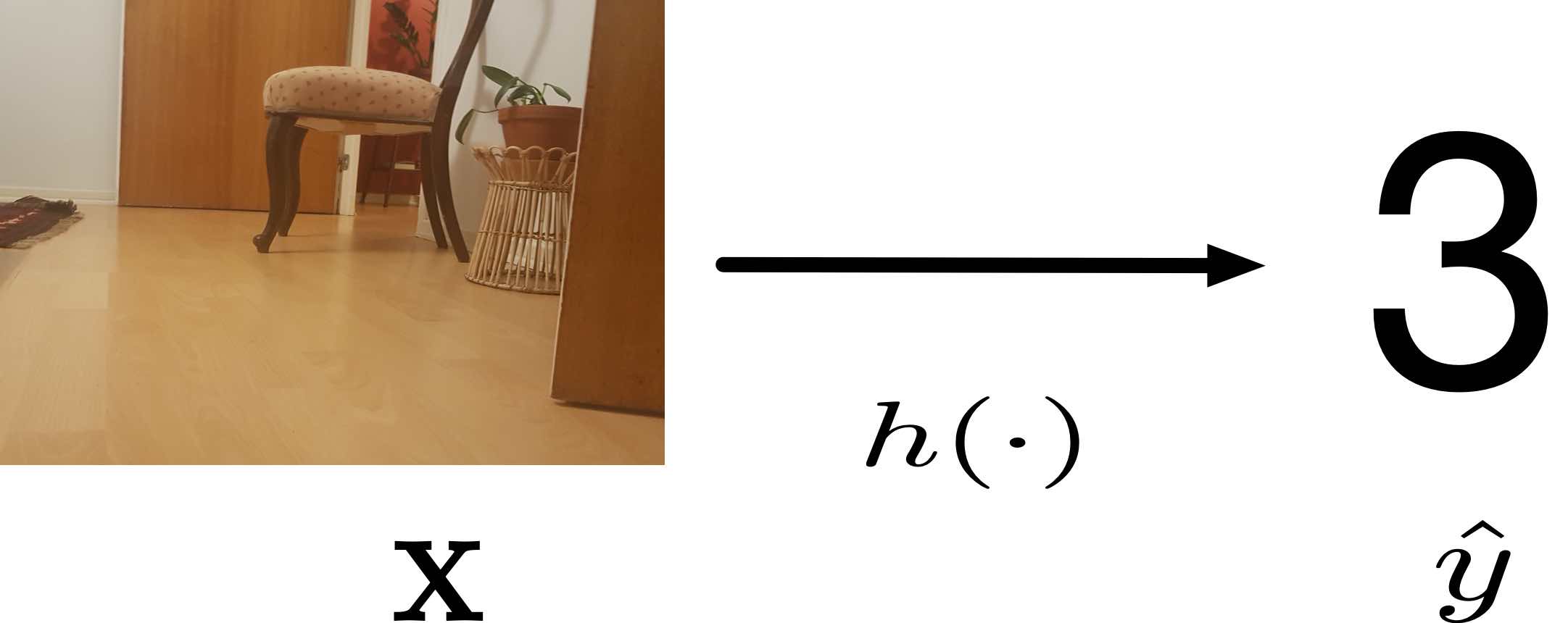
In principle, ML methods could use any possible map [math]h: \featurespace \rightarrow \labelspace[/math] to predict the label [math]\truelabel \in \labelspace[/math] via computing [math]\hat{\truelabel} = h(\featurevec)[/math]. The set of all maps from the feature space [math]\featurespace[/math] to the label space is typically denoted as [math]\labelspace^{\featurespace}[/math].[a]
In general, the set [math]\labelspace^{\featurespace}[/math] is way too large to be search over by a practical ML methods. As a point in case, consider data points characterized by a single numeric feature [math]\feature \in \mathbb{R}[/math] and label [math]\truelabel \in \mathbb{R}[/math]. The set of all real-valued maps [math]h(\feature)[/math] of a real-valued argument already contains uncountably infinite many different hypothesis maps [28].
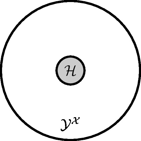
Practical ML methods can search and evaluate only a (tiny) subset of all possible hypothesis maps. This subset of computationally feasible (“affordable”) hypothesis maps is referred to as the hypothesis space or model underlying a ML method. As depicted in Figure fig_hypo_space, ML methods typically use a hypothesis space [math]\hypospace[/math] that is a tiny subset of [math]\labelspace^{\featurespace}[/math]. Similar to the features and labels used to characterize data points, also the hypothesis space underlying a ML method is a design choice. As we will see, the choice for the hypothesis space involves a trade-off between computational complexity and statistical properties of the resulting ML methods.
The preference for a particular hypothesis space often depends on the computational infrastructure that is available to a ML method. Different computational infrastructures favour different hypothesis spaces. ML methods implemented in a small embedded system, might prefer a linear hypothesis space which results in algorithms that require a small number of arithmetic operations. Deep learning methods implemented in a cloud computing environment typically use much larger hypothesis spaces obtained from large artificial neural network (ANN) (see Section Deep Learning ).
ML methods can also be implemented using a spreadsheet software. Here, we might use a hypothesis space consisting of maps [math]h: \featurespace \rightarrow \labelspace[/math] that are represented by look up tables (see Table table-lookup). If we instead use the programming language Python to implement a ML method, we can obtain a hypothesis class by collecting all possible Python subroutines with one input (scalar feature [math]\feature[/math]), one output argument (predicted label [math]\hat{\truelabel}[/math]) and consisting of less than [math]100[/math] lines of code.
| feature x | prediction h(x) |
|---|---|
| 0 | 0 |
| 1/10 | 10 |
| 2/10 | 3 |
| [math]\vdots[/math] | [math]\vdots[/math] |
| 1 | 22.3 |
Broadly speaking, the design choice for the hypothesis space [math]\hypospace[/math] of a ML method has to balance between two conflicting requirements.
- It has to be sufficiently large such that it contains at least one accurate predictor map [math]\hat{h} \in \hypospace[/math]. A hypothesis space [math]\hypospace[/math] that is too small might fail to include a predictor map required to reproduce the (potentially highly non-linear) relation between features and label. Consider the task of grouping or classifying images into “cat” images and “no cat image”. The classification of each image is based solely on the feature vector obtained from the pixel colour intensities. The relation between features and label ([math]\truelabel \in \{ \mbox{cat}, \mbox{no cat} \}[/math]) is highly non-linear. Any ML method that uses a hypothesis space consisting only of linear maps will most likely fail to learn a good predictor (classifier). We say that a ML method is underfitting if it uses a hypothesis space that does not contain any hypotheses maps that can accurately predict the label of any data points.
- It has to be sufficiently small such that its processing fits the available computational resources (memory, bandwidth, processing time). We must be able to efficiently search over the hypothesis space to find good predictors (see Section The Loss and Chapter Empirical Risk Minimization ). This requirement implies also that the maps [math]h(\featurevec)[/math] contained in [math]\hypospace[/math] can be evaluated (computed) efficiently [29]. Another important reason for using a hypothesis space [math]\hypospace[/math] that is not too large is to avoid overfitting (see Chapter Regularization ). If the hypothesis space [math]\hypospace[/math] is too large, then we can easily find a hypothesis which (almost) perfectly predicts the labels of data points in a training set which is used to learn a hypothesis. However, such a hypothesis might deliver poor predictions for labels of data points outside the training set. We say that the hypothesis does not generalize well.
Parametrized Hypothesis spaces
A wide range of current scientific computing environments allow for efficient numerical linear algebra. This hard- and software allows to efficiently process data that is provided in the form of numeric arrays such as vectors, matrices or tensors [1]. To take advantage of such computational infrastructure, many ML methods use the hypothesis space
The hypothesis space \eqref{equ_def_hypo_linear_pred} is constituted by linear maps (functions)
The function [math]h^{(\weights)}[/math] \eqref{equ_def_linear_map} maps, in a linear fashion, the feature vector [math]\featurevec \in \mathbb{R}^{\featuredim}[/math] to the predicted label [math]h^{(\weights)}(\featurevec) = \featurevec^{T} \weights \in \mathbb{R}[/math]. For [math]\featuredim\!=\!1[/math] the feature vector reduces a single feature [math]\feature[/math] and the hypothesis space \eqref{equ_def_hypo_linear_pred} consists of all maps [math]h^{(\weight)}(\feature) = \weight \feature[/math] with weight [math]\weight \in \mathbb{R}[/math] (see Figure scalar_lin_space).
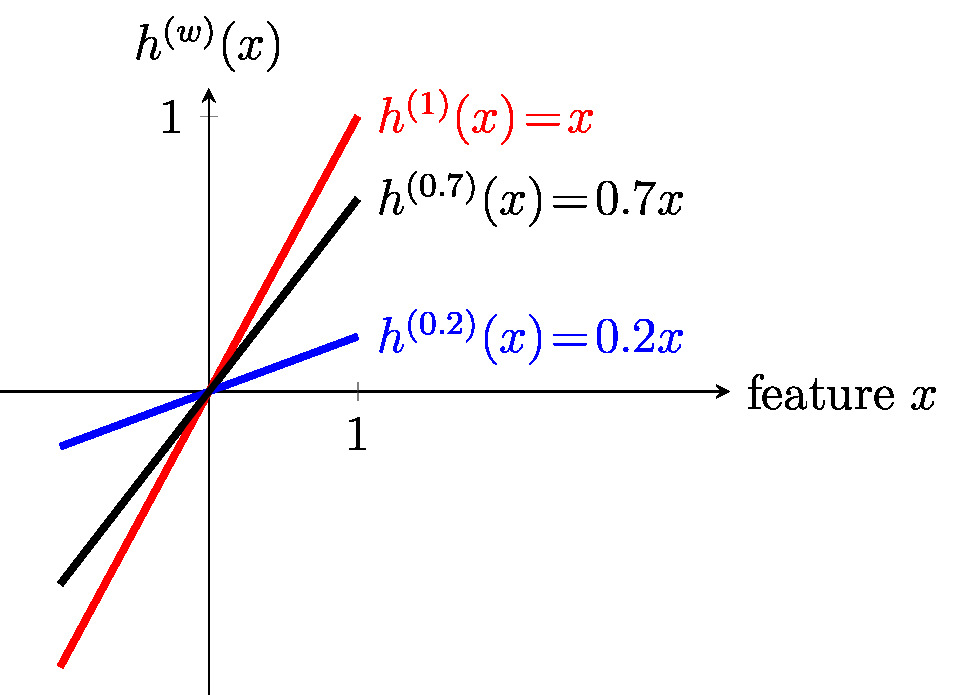
The elements of the hypothesis space [math]\hypospace[/math] in \eqref{equ_def_hypo_linear_pred} are parametrized by the parameter vector [math]\weights \in \mathbb{R}^{\featuredim}[/math]. Each map [math]h^{(\weights)} \in \hypospace[/math] is fully specified by the parameter vector [math]\weights \in \mathbb{R}^{\featuredim}[/math]. This parametrization of the hypothesis space [math]\hypospace[/math] allows to process and manipulate hypothesis maps by vector operations. In particular, instead of searching over the function space [math]\hypospace[/math] (its elements are functions!) to find a good hypothesis, we can equivalently search over all possible parameter vectors [math]\weights \in \mathbb{R}^{\featuredim}[/math].
The search space [math]\mathbb{R}^{\featuredim}[/math] is still (uncountably) infinite but it has a rich geometric and algebraic structure that allows to efficiently search over this space. Chapter Gradient-Based Learning discusses methods that use the concept ot a gradient to implement an efficient search for useful parameter vectors [math]\weights \in \mathbb{R}^{\featurelen}[/math].
The hypothesis space \eqref{equ_def_hypo_linear_pred} is also appealing because of the broad availability of computing hardware such as graphic processing units. Another factor boosting the widespread use of \eqref{equ_def_hypo_linear_pred} might be the offer for optimized software libraries for numerical linear algebra.
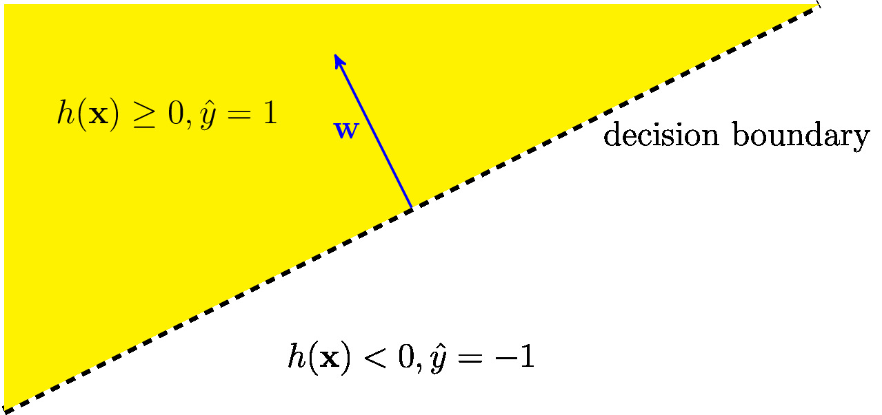
The hypothesis space \eqref{equ_def_hypo_linear_pred} can also be used for classification problems, e.g., with label space [math]\labelspace = \{-1,1\}[/math]. Indeed, given a linear predictor map [math]h^{(\weights)}[/math] we can classify data points according to [math]\hat{\truelabel}\!=\!1[/math] for [math]h^{(\weights)}(\featurevec) \geq 0[/math] and [math]\hat{\truelabel}\!=\!-1[/math] otherwise. We refer to a classifier that computes the predicted label by first applying a linear map to the features as a linear classifier.
Figure fig_lin_dec_boundary illustrates the decision regions \eqref{equ_decision_region} of a linear classifier for binary labels. The decision regions are half-spaces and, in turn, the decision boundary is a hyperplane [math]\{ \featurevec: \weights^{T} \featurevec = b \}[/math]. Note that each linear classifier corresponds to a particular linear hypothesis map from the hypothesis space \eqref{equ_def_hypo_linear_pred}. However, we can use different loss functions to measure the quality of a linear classifier. Three widely-used examples for ML methods that learn a linear classifier are logistic regression (see Section Logistic Regression ), the support vector machine (SVM) (see Section Support Vector Machines ) and the naive Bayes classifier (see Section Bayes Classifier ).
In some application domains, the relation between features [math]\featurevec[/math] and label [math]\truelabel[/math] of a data point is highly non-linear. As a case in point, consider data points that are images of animals. The map that relates the pixel intensities of an image to a label value indicating if the image shows a cat is highly non-linear. For such applications, the hypothesis space \eqref{equ_def_hypo_linear_pred} is not suitable as it only contains linear maps. The second main example for a parametrized hypothesis space studied in this book contains also non-linear maps. This parametrized hypothesis space is obtained from a parametrized signal flow diagram which is referred to as an ANN. Section Deep Learning discusses the construction of non-linear parametrized hypothesis spaces using an ANN.
Upgrading a Hypothesis Space via Feature Maps. Let us discuss a simple but powerful technique for enlarging (“upgrading”) a given hypothesis space [math]\hypospace[/math] to a larger hypothesis space [math]\hypospace' \supseteq \hypospace[/math] that offers a wider selection of hypothesis maps. The idea is to replace the original features [math]\featurevec[/math] of a data point with new (transformed) features [math]\rawfeaturevec = \featuremapvec (\featurevec)[/math]. The transformed features are obtained by applying a feature map [math]\featuremap(\cdot)[/math] to the original features [math]\featurevec[/math]. This upgraded hypothesis space [math]\hypospace'[/math] consists of all concatenations of the feature map [math]\featuremap[/math] and some hypothesis [math]h \in \hypospace[/math],
The construction \eqref{equ_def_enlarged_hypospace} used for arbitrary combinations of a feature map [math]\featuremap(\cdot)[/math] and a “base” hypothesis space [math]\hypospace[/math]. The only requirement is that the output of the feature map can be used as input for a hypothesis [math]h \in \hypospace[/math]. More formally, the range of the feature map must belong to the domain of the maps in [math]\hypospace[/math]. Examples for ML methods that use a hypothesis space of the form \eqref{equ_def_enlarged_hypospace} include polynomial regression (see Section Polynomial Regression ), Gaussian basis regression (see Section Gaussian Basis Regression ) and the important family of kernel methods (see Section Kernel Methods ). The feature map in \eqref{equ_def_enlarged_hypospace} might also be obtained from clustering or feature learning methods (see Section Clustering as Preprocessing and Section Combining PCA with linear regression).
For the special case of the linear hypothesis space \eqref{equ_def_hypo_linear_pred}, the resulting enlarged hypothesis space \eqref{equ_def_enlarged_hypospace} is given by all linear maps [math]\weights^{T} \rawfeaturevec[/math] of the transformed features [math]\featuremapvec(\featurevec)[/math]. Combining the hypothesis space \eqref{equ_def_hypo_linear_pred} with a non-linear feature map results in a hypothesis space that contains non-linear maps from the original feature vector [math]\featurevec[/math] to the predicted label [math]\hat{\truelabel}[/math],
Non-Numeric Features.
The hypothesis space \eqref{equ_def_hypo_linear_pred} can only be used for data points whose features are numeric vectors [math]\featurevec = (\feature_{1},\ldots,\feature_{\featuredim})^{T} \in \mathbb{R}^{\featuredim}[/math]. In some application domains, such as natural language processing, there is no obvious natural choice for numeric features. However, since ML methods based on the hypothesis space \eqref{equ_def_hypo_linear_pred} are well developed (using numerical linear algebra),
it might be useful to construct numerical features even for non-numeric data (such as text). For text data, there has been significant progress recently on methods that map a human-generated text into sequences of vectors (see [30](Chap. 12) for more details). Moreover, Section Feature Learning for Non-Numeric Data will discuss an approach to generate numeric features for data points that have an intrinsic notion of similarity.
The Size of a Hypothesis Space
The notion of a hypothesis space being too small or being too large can be made precise in different ways. The size of a finite hypothesis space [math]\hypospace[/math] can be defined as its cardinality [math]|\hypospace|[/math] which is simply the number of its elements. For example, consider data points represented by [math]100 \times 10\!=\!1000[/math] black-and-white pixels and characterized by a binary label [math]\truelabel \in \{0,1\}[/math]. We can model such data points using the feature space [math]\featurespace = \{0,1\}^{1000}[/math] and label space [math]\labelspace = \{0,1\}[/math]. The largest possible hypothesis space [math]\hypospace = \labelspace^\featurespace[/math] consists of all maps from [math]\featurespace[/math] to [math]\labelspace[/math]. The size or cardinality of this space is [math]|\hypospace| = 2^{2^{1000}}[/math].
Many ML methods use a hypothesis space which contains infinitely many different predictor maps (see, e.g., \eqref{equ_def_hypo_linear_pred}). For an infinite hypothesis space, we cannot use the number of its elements as a measure for its size. Indeed, for an infinite hypothesis space, the number of elements is not well-defined. Therefore, we measure the size of a hypothesis space [math]\hypospace[/math] using its effective dimension [math]\effdim{\hypospace}[/math].
Consider a hypothesis space [math]\hypospace[/math] consisting of maps [math]h: \featurespace\rightarrow \labelspace[/math] that read in the features [math]\featurevec \in \featurespace[/math] and output an predicted label [math]\hat{\truelabel} = h(\featurevec) \in \labelspace[/math]. We define the effective dimension [math]\effdim{\hypospace}[/math] of [math]\hypospace[/math] as the maximum number [math]\sizehypospace \in \mathbb{N}[/math] such that for any set [math]\dataset = \big\{ \big(\featurevec^{(1)},\truelabel^{(1)}\big), \ldots, \big(\featurevec^{(\sizehypospace)},\truelabel^{(\sizehypospace)}\big) \}[/math] of [math]\sizehypospace[/math] data points with different features, we can always find a hypothesis [math]h \in \hypospace[/math] that perfectly fits the labels, [math]\truelabel^{(\sampleidx)} = h\big( \featurevec^{(\sampleidx)} \big)[/math] for [math]\sampleidx=1,\ldots,\sizehypospace[/math].
The effective dimension of a hypothesis space is closely related to the Vapnik–Chervonenkis (VC) dimension [31]. The VC dimension is maybe the most widely used concept for measuring the size of infinite hypothesis spaces [31][32][25][33]. However, the precise definition of the VC dimension are beyond the scope of this book. Moreover, the effective dimension captures most of the relevant properties of the VC dimension for our purposes. For a precise definition of the VC dimension and discussion of its applications in ML we refer to [32]. Let us illustrate the concept of effective dimension as a measure for the size of a hypothesis space with two examples: linear regression and polynomial regression.
Linear regression uses the hypothesis space [math]\hypospace^{(\featuredim)} = \{ h: \mathbb{R}^{\featuredim} \rightarrow \mathbb{R}: h(\featurevec) = \weights^{T} \featurevec \mbox{ with some vector } \weights \in \mathbb{R}^{\featurelen}\}.[/math] Consider a dataset [math]\dataset=\big\{ \big(\featurevec^{(1)} ,\truelabel^{(1)}\big),\ldots, \big(\featurevec^{(\samplesize)} ,\truelabel^{(\samplesize)}\big) \big\} [/math] consisting of [math]\samplesize[/math] data points. We refer to this number also as the sample size of the dataset. Each data point is characterized by a feature vector [math]\featurevec^{(\sampleidx)} \in \mathbb{R}^{\featuredim}[/math] and a numeric label [math]\truelabel^{(\sampleidx)} \in \mathbb{R}[/math]. Let us further assume that data points are realizations of iid RVs with a common probability distribution.
Under the i.i.d. assumption, the matrix [math]\featuremtx = \big(\featurevec^{(1)},\ldots,\featurevec^{(\samplesize)}\big) \in \mathbb{R}^{\featuredim\times \samplesize},[/math] which is obtained by stacking (column-wise) the feature vectors [math]\featurevec^{(\sampleidx)}[/math] (for [math]\sampleidx=1,\ldots,\samplesize[/math]), is full (column-) rank with probability one. Basic results of linear algebra allow to show that the data points in [math]\dataset[/math] can be perfectly fit by a linear map [math]h \in \hypospace^{(\featuredim)}[/math] as long as [math]\samplesize \leq \featuredim[/math].
As long as the number [math]\samplesize[/math] of data points does not exceed the number of features characterizing each data point, i.e., as long as [math]\samplesize \leq \featuredim[/math], we can find (with probability one) a parameter vector [math]\widehat{\weights}[/math] such that [math]\truelabel^{(\sampleidx)} = \widehat{\weights}^{T} \featurevec^{(\sampleidx)}[/math] for all [math]\sampleidx=1,\ldots,\samplesize[/math]. The effective dimension of the linear hypothesis space [math]\hypospace^{(\featuredim)}[/math] is therefore [math]\sizehypospace = \featuredim[/math].
As a second example, consider the hypothesis space [math]\hypospace_{\rm poly}^{(\featuredim)}[/math] which is constituted by the set of polynomials with maximum degree [math]\featuredim[/math]. The fundamental theorem of algebra tells us that any set of [math]\samplesize[/math] data points with different features can be perfectly fit by a polynomial of degree [math]\featuredim[/math] as long as [math]\featuredim \geq \samplesize[/math]. Therefore, the effective dimension of the hypothesis space [math]\hypospace_{\rm poly}^{(\featuredim)}[/math] is [math]\sizehypospace=\featuredim[/math]. Section Polynomial Regression discusses polynomial regression in more detail.
The Loss
Every ML method uses a (more of less explicit) hypothesis space [math]\hypospace[/math] which consists of all computationally feasible predictor maps [math]h[/math]. Which predictor map [math]h[/math] out of all the maps in the hypothesis space [math]\hypospace[/math] is the best for the ML problem at hand? To answer this questions, ML methods use the concept of a loss function. Formally, a loss function is a map [math]\lossfun: \featurespace \times \labelspace \times \hypospace \rightarrow \mathbb{R}_{+}: \big( \big(\featurevec,\truelabel\big), h\big) \mapsto \loss{(\featurevec,\truelabel)}{h}[/math] which assigns a pair consisting of a data point, itself characterized by features [math]\featurevec[/math] and label [math]\truelabel[/math], and a hypothesis [math]h \in \hypospace[/math] the non-negative real number [math]\loss{(\featurevec,\truelabel)}{h}[/math].
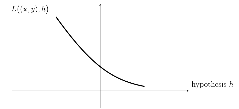
The loss value [math]\loss{(\featurevec,\truelabel)}{h}[/math] quantifies the discrepancy between the true label [math]\truelabel[/math] and the predicted label [math]h(\featurevec)[/math]. A small (close to zero) value [math]\loss{(\featurevec,\truelabel)}{h}[/math] indicates a low discrepancy between predicted label and true label of a data point. Figure fig_loss_function depicts a loss function for a given data point, with features [math]\featurevec[/math] and label [math]\truelabel[/math], as a function of the hypothesis [math]h \in \hypospace[/math]. The basic principle of ML methods can then be formulated as: Learn (find) a hypothesis out of a given hypothesis space [math]\hypospace[/math] that incurs a minimum loss [math]\loss{(\featurevec,\truelabel)}{h}[/math] for any data point (see Chapter Empirical Risk Minimization ).
Much like the choice for the hypothesis space [math]\hypospace[/math] used in a ML method, also the loss function is a design choice. We will discuss some widely used examples for loss function in Section Loss Functions for Numeric Labels and Section Loss Functions for Categorical Labels. The choice for the loss function should take into account the computational complexity of searching the hypothesis space for a hypothesis with minimum loss. Consider a ML method that uses a parametrized hypothesis space and a loss function that is a convex and differentiable (smooth) function of the parameters of a hypothesis. In this case, searching for a hypothesis with small loss can be done efficiently using the gradient-based methods discussed in Chapter Gradient-Based Learning . The minimization of a loss function that is either non-convex or non-differentiable is typically computationally much more difficult. Section Computational and Statistical Aspects of ERM discusses the computational complexities of different types of loss functions in more detail.
Beside computational aspects, the choice for the loss function should also take into account statistical aspects. For example, some loss functions result in ML methods that are more robust against outliers (see Section Least Absolute Deviation Regression and Section Support Vector Machines ). The choice of loss function might also be guided by probabilistic models for the data generated in an ML application. Section Maximum Likelihood details how the maximum likelihood principle of statistical inference provides an explicit construction of loss functions in terms of an (assumed) probability distribution for data points.
The choice for the loss function used to evaluate the quality of a hypothesis might also be influenced by its interpretability. Section Loss Functions for Categorical Labels discusses loss functions for hypotheses that are used to classify data points into two categories. It seems natural to measure the quality of such a hypothesis by the average number of wrongly classified data points, which is precisely the average [math]0/1[/math] loss \eqref{equ_def_0_1} (see Section Loss Functions for Categorical Labels).
In contrast to its appealing interpretation as error-rate, the computational aspects of the average [math]0/1[/math] loss are less pleasant. Minimizing the average [math]0/1[/math] loss to learn an accurate hypothesis amounts to a non-convex and non-smooth optimization problem which is computationally challenging. Section Loss Functions for Categorical Labels introduces the logistic loss as a computationally attractive alternative choice for the loss function in binary classification problems. Learning a hypothesis that minimizes a (average) logistic loss amounts to a smooth convex optimization problem. Chapter Gradient-Based Learning discusses computationally cheap gradient-based methods for solving smooth convex optimization problems.
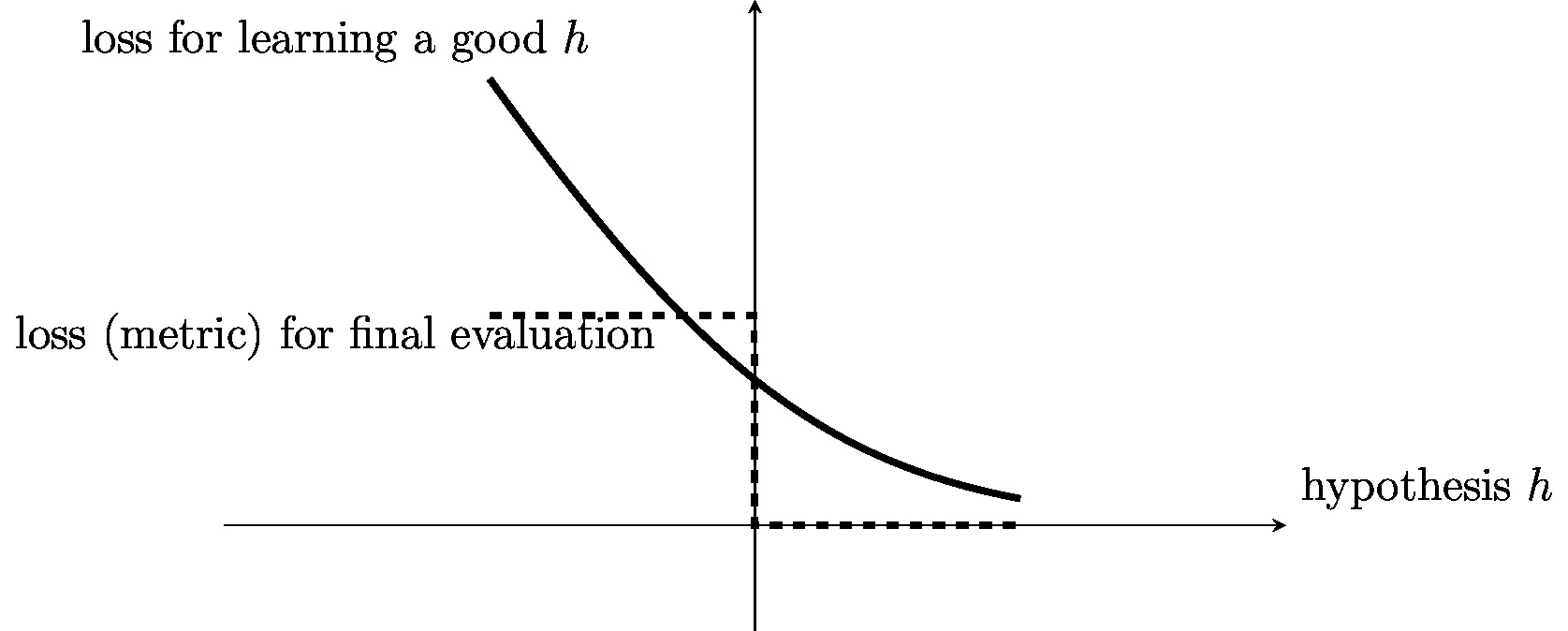
The above aspects (computation, statistic, interpretability) result typically in conflicting goals for the choice of a loss function. A loss function that has favourable statistical properties might incur a high computational complexity of the resulting ML method. Loss functions that result in computationally efficient ML methods might not allow for an easy interpretation (what does it mean intuitively if the logistic loss of a hypothesis in a binary classification problem is [math]10^{-1}[/math]?). It might therefore be useful to use different loss functions for the search of a good hypothesis (see Chapter Empirical Risk Minimization ) and for its final evaluation. Figure fig_loss_function_and_metric depicts an example for two such loss functions, one of them used for learning a hypothesis by minimizing the loss and the other one used for the final performance evaluation.
For example, in a binary classification problem, we might use the logistic loss to search for (learn) an accurate hypothesis using the optimization methods in Chapter Empirical Risk Minimization . The logistic loss is appealing for this purpose as it can be minimized via efficient gradient-based methods (see Chapter Gradient-Based Learning ). After having found (learnt) an accurate hypothesis, we use the average [math]0/1[/math] loss for the final performance evaluation. The [math]0/1[/math] loss is appealing for this purpose as it can be interpreted as an error or misclassification rate. The loss function used for the final performance evaluation of a learnt hypothesis is sometimes referred to as metric.
Loss Functions for Numeric Labels
For ML problems involving data points with a numeric label [math]\truelabel \in \mathbb{R}[/math], i.e., for regression problems (see Section Labels), a widely used (first) choice for the loss function can be the squared error loss
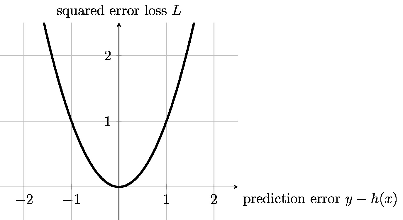
The squared error loss \eqref{equ_squared_loss} depends on the features [math]\featurevec[/math] only via the predicted label value [math]\predictedlabel= h(\featurevec)[/math]. We can evaluate the squared error loss solely using the prediction [math]h(\featurevec)[/math] and the true label value [math]\truelabel[/math]. Besides the prediction [math]h(\featurevec)[/math], no other properties of the features [math]\featurevec[/math] are required to determine the squared error loss. We will slightly abuse notation and use the shorthand [math]\loss{\truelabel}{\predictedlabel}[/math] for any loss function that depends on the features [math]\featurevec[/math] only via the predicted label [math]\predictedlabel=h(\featurevec)[/math]. Figure fig_squarederror_loss depicts the squared error loss as a function of the prediction error [math]\truelabel - \predictedlabel[/math].
The squared error loss \eqref{equ_squared_loss} has appealing computational and statistical properties. For linear predictor maps [math]h(\featurevec) = \weights^{T} \featurevec[/math], the squared error loss is a convex and differentiable function of the parameter vector [math]\weights[/math]. This allows, in turn, to efficiently search for the optimal linear predictor using efficient iterative optimization methods (see Chapter Gradient-Based Learning ). The squared error loss also has a useful interpretation in terms of a probabilistic model for the features and labels. Minimizing the squared error loss is equivalent to maximum likelihood estimation within a linear Gaussian model [33] (Sec. 2.6.3).
Another loss function used in regression problems is the absolute error loss [math]|\hat{y} - y|[/math]. Using this loss function to guide the learning of a predictor results in methods that are robust against a few outliers in the training set (see Section Least Absolute Deviation Regression ). However, this improved robustness comes at the expense of increased computational complexity of minimizing the (non-differentiable) absolute error loss compared to the (differentiable) squared error loss \eqref{equ_squared_loss}.
Loss Functions for Categorical Labels
Classification problems involve data points whose labels take on values from a discrete label space [math]\labelspace[/math]. In what follows, unless stated otherwise, we focus on binary classification problems. Moreover, without loss of generality, we use the label space [math]\labelspace = \{-1,1\}[/math]. Classification methods aim at learning a hypothesis or classifier that maps the features [math]\featurevec[/math] of a data point to a predicted label [math]\hat{\truelabel} \in \labelspace[/math].
It is often convenient to implement a classifier by thresholding the value [math]h(\featurevec) \in \mathbb{R}[/math] of a hypothesis map that can deliver arbitrary real numbers. We then classify a data point as [math]\predictedlabel=1[/math] if [math]h(\featurevec)\gt0[/math] and [math]\predictedlabel=-1[/math] otherwise. Thus, the predicted label is obtained from the sign of the value [math]h(\featurevec)[/math]. While the sign of [math]h(\featurevec)[/math] determines the predicted label [math]\predictedlabel[/math], we can interpret the absolute value [math]|h(\featurevec)|[/math] as the confidence in this classification. Is is customary to abuse notation and refer to both, the final classification rule (obtained by a thresholding step) [math]\featurevec \mapsto \predictedlabel[/math] and the hypothesis [math]h(\featurevec)[/math] (whose outout is thresholded) as a binary classifier.
In principle, we can measure the quality of a hypothesis when used to classify data points using the squared error loss \eqref{equ_squared_loss}. However, the squared error is typically a poor measure for the quality of a hypothesis [math]h(\featurevec)[/math] that is used to classify a data point with binary label [math]\truelabel \in \{-1,1\}[/math]. Figure fig_squarederrornotgoodclass illustrates how the squared error loss of a hypothesis can be (highly) misleading for binary classification.
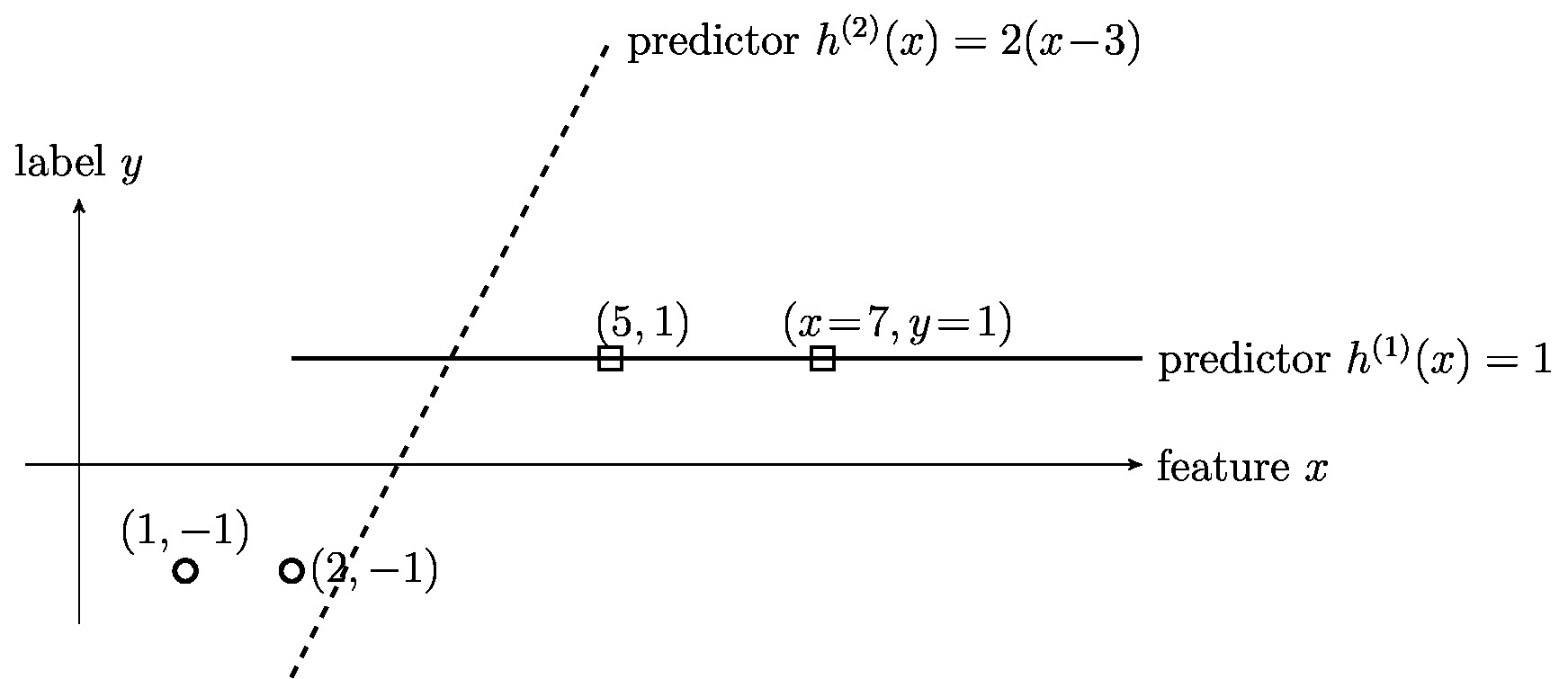
Figure fig_squarederrornotgoodclass depicts a dataset [math]\dataset[/math] consisting of [math]\samplesize=4[/math] data points with binary labels [math]\truelabel^{(\sampleidx)} \in \{-1,1\}[/math], for [math]\sampleidx=1,\ldots,\samplesize[/math]. The figure also depicts two candidate hypotheses [math]h^{(1)}(\feature)[/math] and [math]h^{(2)}(\feature)[/math] that can be used for classifying data points. The classifications [math]\predictedlabel[/math] obtained with the hypothesis [math]h^{(2)}(\feature)[/math] would perfectly match the labels of the four training data points since [math]h^{(2)}\big(\feature^{(\sampleidx)}\big)\geq 0[/math] if and if only if [math]\truelabel^{(\sampleidx)}=1[/math]. In contrast, the classifications [math]\predictedlabel^{(\sampleidx)}[/math] obtained by thresholding [math]h^{(1)}(\feature)[/math] are wrong for data points with [math]\truelabel=-1[/math].
Looking at [math]\dataset[/math], we might prefer using [math]h^{(2)}(\feature)[/math] over [math]h^{(1)}[/math] to classify data points. However, the squared error loss incurred by the (reasonable) classifier [math]h^{(2)}[/math] is much larger than the squared error loss incurred by the (poor) classifier [math]h^{(1)}[/math]. The squared error loss is typically a bad choice for assessing the quality of a hypothesis map that is used for classifying data points into different categories.
Generally speaking, we want the loss function to punish (deliver large values for) a hypothesis that is very confident ([math]|h(\featurevec)|[/math] is large) in a wrong classification ([math]\predictedlabel \neq \truelabel[/math]). Moreover, a useful loss function loss function should not punish (deliver small values for) a hypothesis is very confident ([math]|h(\featurevec)|[/math] is large) in a correct classification ([math]\predictedlabel = \truelabel[/math]). However, by its very definition, the squared loss \eqref{equ_squared_loss} yields large values if the confidence [math]|h(\featurevec)|[/math] is large, no matter if the resulting (after thresholding) classification is correct or wrong.
We now discuss some loss functions which have proven useful for assessing the quality of a hypothesis that is used to classify data points. Unless noted otherwise, the formulas for these loss functions are valid only if the label values are the real numbers [math]-1[/math] and [math]1[/math] (the label space is [math]\labelspace = \{-1,1\}[/math]). These formulas need to modified accordingly if different label values are used. For example, instead of the label space [math]\labelspace = \{-1,1\}[/math], we could equally well use the label space [math]\labelspace =\{0,1\}[/math], or [math]\labelspace = \{ \square, \triangle \}[/math] or [math]\labelspace = \{ \mbox{ “Class 1”}, \mbox{ “Class 2”} \}[/math].
A natural choice for the loss function can be based on the requirement that a reasonable hypothesis should deliver a correct classifications, [math]\predictedlabel = \truelabel[/math] for any data point. This suggests to learn a hypothesis [math]h(\featurevec)[/math] by minimizing the [math]0/1[/math] loss
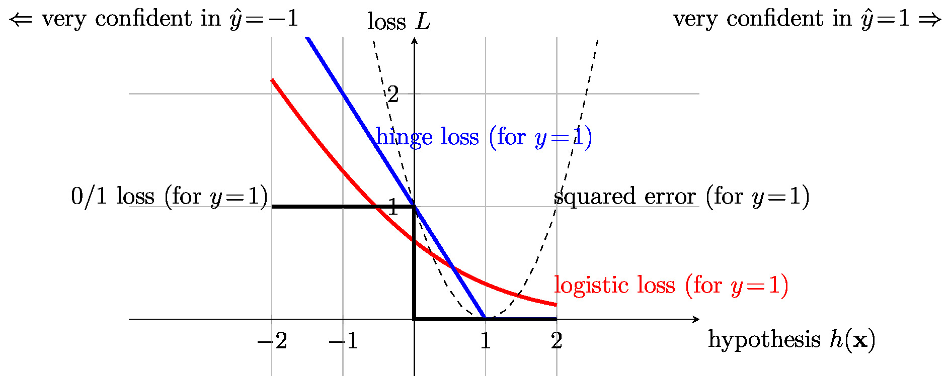
Figure fig_class_loss illustrates the [math]0/1[/math] loss \eqref{equ_def_0_1} for a data point with features [math]\featurevec[/math] and label [math]\truelabel\!=\!1[/math] as a function of the hypothesis value [math]h(\featurevec)[/math]. The [math]0/1[/math] loss is equal to zero if the hypothesis yields a correct classification [math]\predictedlabel=\truelabel[/math]. For a wrong classification [math]\predictedlabel\neq\truelabel[/math], the [math]0/1[/math] loss yields the value one.
The [math]0/1[/math] loss \eqref{equ_def_0_1} is conceptually appealing when data points are interpreted as realizations of iid RVs with the same probability distribution [math]p(\featurevec,\truelabel)[/math]. Given [math]\samplesize[/math] realizations [math](\featurevec^{(\sampleidx)},\truelabel^{(\sampleidx)}) \big\}_{\sampleidx=1}^{\samplesize}[/math] of such iid RVs,
with high probability for sufficiently large sample size [math]\samplesize[/math]. A precise formulation of the approximation \eqref{equ_0_1_approx_prob} can be obtained from the law of large numbers [24](Section 1). We can apply the law of large numbers since the loss values [math]\loss{(\featurevec^{(\sampleidx)},\truelabel^{(\sampleidx)})}{h}[/math] are realizations of iid RVs. It is customary to indicate the average [math]0/1[/math] loss of a hypothesis as the accuracy [math]1 - (1/\samplesize) \sum_{\sampleidx=1}^{\samplesize} \loss{(\featurevec^{(\sampleidx)},\truelabel^{(\sampleidx)})}{h}[/math].
In view of \eqref{equ_0_1_approx_prob}, the [math]0/1[/math] loss \eqref{equ_def_0_1} seems a very natural choice for assessing the quality of a classifier if our goal is to enforce correct classifications [math]\hat{\truelabel}=\truelabel[/math]. This appealing statistical property of the [math]0/1[/math] loss comes at the cost of a high computational complexity. Indeed, for a given data point [math](\featurevec,\truelabel)[/math], the [math]0/1[/math] loss \eqref{equ_def_0_1} is non-convex and non-differentiable when viewed as a function of the hypothesis [math]h[/math]. Thus, ML methods that use the [math]0/1[/math] loss to learn a hypothesis map typically involve advanced optimization methods to solve the resulting learning problem (see Section Bayes Classifier ).
To avoid the non-convexity of the [math]0/1[/math] loss \eqref{equ_def_0_1} we might approximate it by a convex loss function. One popular convex approximation of the [math]0/1[/math] loss is the hinge loss
Figure fig_class_loss depicts the hinge loss \eqref{equ_hinge_loss} as a function of the hypothesis [math]h(\featurevec)[/math]. The hinge loss \eqref{equ_hinge_loss} becomes minimal (equal to zero) for a correct classification ([math]\hat{\truelabel} = \truelabel[/math]) with sufficient confidence [math]h(\featurevec) \geq 1[/math]. For a wrong classification ([math]\hat{\truelabel} \neq \truelabel[/math]), the hinge loss increases monotonically with the confidence [math]|h(\feature)|[/math] in the wrong classification. While the hinge loss avoids the non-convexity of the [math]0/1[/math] loss, it still is a non-differentiable function of [math]h(\featurevec)[/math]. A non-differentiable loss function cannot be minimized by simple gradient-based methods (see Chapter Gradient-Based Learning ) but require more advanced optimization methods.
Beside the [math]0/1[/math] loss and the hinge loss, another popular loss function for binary classification problems is the logistic loss
The logistic loss \eqref{equ_log_loss} is used in logistic regression (see Section Logistic Regression ) to measure the usefulness of a linear hypothesis [math]h(\featurevec) = \weights^{T} \featurevec[/math]. Figure fig_class_loss depicts the logistic loss \eqref{equ_log_loss} as a function of the hypothesis [math]h(\featurevec)[/math]. The logistic loss \eqref{equ_log_loss} is a convex and differentiable function of [math]h(\featurevec)[/math]. For a correct classification ([math]\hat{\truelabel}\!=\!\truelabel[/math]), the logistic loss \eqref{equ_log_loss} decreases monotonically with increasing confidence [math]h(\featurevec)[/math]. For a wrong classification ([math]\hat{\truelabel}\!\neq\!\truelabel[/math]), the logistic loss increases monotonically with increasing confidence [math]|h(\featurevec)|[/math] in the wrong classification.
Both the hinge loss \eqref{equ_hinge_loss} and the logistic loss \eqref{equ_log_loss} are convex functions of the weights [math]\weights \in \mathbb{R}^{\featuredim}[/math] in a linear hypothesis map [math]h(\featurevec) = \weights^{T} \featurevec[/math]. However, in contrast to the hinge loss, the logistic loss \eqref{equ_log_loss} is also a differentiable function of the [math]\weights[/math]. The convex and differentiable logistic loss function can be minimized using simple gradient-based methods such as gradient descent (GD) (see Chapter GD for Logistic Regression ). In contrast, we cannot use basic gradient-based methods to minimize the hinge loss since it is not differentiable (it does not have a gradient everywhere). However, we can apply a generalization of GD which is known as subgradient descent [34]. Subgradient descent is obtained from GD by generalizing the concept of a gradient to that of a subgradient.
Loss Functions for Ordinal Label Values
Some loss functions are particularly suited for predicting ordinal label values (see Section The Data ). Consider data points representing areal images of rectangular areas of size [math]1 \mbox{km}[/math] by [math]1 \mbox{km}[/math]. We characterize each data point (rectangular area) by the feature vector [math]\featurevec[/math] obtained by stacking the RGB values of each image pixel (see Figure fig_snapshot_pixels). Beside the feature vector, each rectangular area is characterized by a label [math]\truelabel \in \{1,2,3\}[/math] where
- [math]\truelabel=1[/math] means that the area contains no trees.
- [math]\truelabel=2[/math] means that the area is partially covered by trees.
- [math]\truelabel=3[/math] means that the are is entirely covered by trees.
We might consider the label value [math]\truelabel=2[/math] to be “larger” than label value [math]\truelabel=1[/math] and label value [math]\truelabel=3[/math] to be “larger” than label value [math]\truelabel=2[/math]. Let us construct a loss function that takes such an ordering of label values into account when evaluating the quality of the predictions [math]h(\featurevec)[/math].
Consider a data point with feature vector [math]\featurevec[/math] and label [math]\truelabel=1[/math] as well as two different hypotheses [math]h^{(a)}, h^{(b)} \in \hypospace[/math]. The hypothesis [math]h^{(a)}[/math] delivers the predicted label [math]\hat{\truelabel}^{(a)}= h^{(a)}(\featurevec) =2[/math], while the other hypothesis [math]h^{(b)}[/math] delivers the predicted label [math]\hat{\truelabel}^{(a)}= h^{(a)}(\featurevec) =3[/math]. Both predictions are wrong, since they are different form the true label value [math]\truelabel=1[/math]. It seems reasonable to consider the prediction [math]\hat{\truelabel}^{(a)}[/math] to be less wrong than the prediction [math]\hat{\truelabel}^{(b)}[/math] and therefore we would prefer the hypothesis [math]h^{(a)}[/math] over [math]h^{(b)}[/math]. However, the [math]0/1[/math] loss is the same for [math]h^{(a)}[/math] and [math]h^{(b)}[/math] and therefore does not reflect our preference for [math]h^{(a)}[/math]. We need to modify (or tailor) the [math]0/1[/math] loss to take into account the application-specific ordering of label values. For the above application, we might define a loss function via
Empirical Risk
The basic idea of ML methods (including those discussed in Chapter The Landscape of ML ) is to find (or learn) a hypothesis (out of a given hypothesis space [math]\hypospace[/math]) that incurs minimum loss when applied to arbitrary data points. To make this informal goal precise we need to specify what we mean by “arbitrary data point”.
One of the most successful approaches to define the notion of “arbitrary data point” is by probabilistic models for the observed data points. The most basic and widely-used probabilistic model interprets data points [math]\big( \featurevec^{(\sampleidx)},\truelabel^{(\sampleidx)} \big)[/math] as realizations of iid RVs with a common probability distribution [math]p(\featurevec,\truelabel)[/math]. Given such a probabilistic model, it seems natural to measure the quality of a hypothesis [math]h[/math] by the expected loss or Bayes risk [21]
The Bayes risk of [math]h[/math] is the expected value of the loss [math]\loss{(\featurevec,\truelabel)}{h}[/math] incurred when applying the hypothesis [math]h[/math] to (the realization of) a random data point with features [math]\featurevec[/math] and label [math]\truelabel[/math]. Note that the computation of the Bayes risk \eqref{equ_def_bayes_risk_int} requires the joint probability distribution [math]p(\featurevec,\truelabel)[/math] of the (random) features and label of data points.
The Bayes risk \eqref{equ_def_bayes_risk_int} seems to be reasonable performance measure for a hypothesis [math]h[/math]. Indeed, the Bayes risk of a hypothesis is small only if the hypothesis incurs a small loss on average for data points drawn from the probability distribution [math]p(\featurevec,\truelabel)[/math]. However, it might be challenging to verify if the data points generated in a particular application domain can be accurately modelled as realizations (draws) from a probability distribution [math]p(\featurevec,\truelabel)[/math]. Moreover, it is also often the case that we do not know the correct probability distribution [math]p(\featurevec,\truelabel)[/math].
Let us assume for the moment, that data points are generated as iid realizations of a common probability distribution [math]p(\featurevec,\truelabel)[/math] which is known. It seems reasonable to learn a hypothesis [math]\bayeshypothesis[/math] that incurs minimum Bayes risk,
A hypothesis that solves \eqref{equ_def_bayes_risk_int}, i.e., that achieves the minimum possible Bayes risk, is referred to as a Bayes estimator [21](Chapter 4). The main computational challenge for learning the optimal hypothesis is the efficient (numerical) solution of the optimization problem \eqref{equ_def_bayes_risk_int}. Efficient methods to solve the optimization problem \eqref{equ_def_bayes_risk_int} are studied within estimation theory [21][35].
The focus of this book is on ML methods which do not require knowledge of the underlying probability distribution [math]p(\featurevec,\truelabel)[/math]. One of the most widely used principle for these ML methods is to approximate the Bayes risk by an empirical (sample) average over a finite set of labeled data points [math]\dataset=\big(\featurevec^{(1)},\truelabel^{(1)}\big),\ldots,\big(\featurevec^{(\samplesize)},\truelabel^{(\samplesize)}\big)[/math]. In particular, we define the empirical risk of a hypothesis [math]h \in \hypospace[/math] for a dataset [math]\dataset[/math] as
The empirical risk of the hypothesis [math]h \in \hypospace[/math] is the average loss on the data points in [math]\dataset[/math]. To ease notational burden, we use [math]\emperror(h)[/math] as a shorthand for [math]\emperror(h|\dataset)[/math] if the underlying dataset [math]\dataset[/math] is clear from the context. Note that in general the empirical risk depends on both, the hypothesis [math]h[/math] and the (features and labels of the) data points in the dataset [math]\dataset[/math].
If the data points used to compute the empirical risk \eqref{eq_def_emp_error_101} are (can be modelled as) realizations of iid RVs whose common distribution is [math]p(\featurevec,\truelabel)[/math], basic results of probability theory tell us that
The approximation error in \eqref{equ_emp_risk_approximates_Bayes_risk} can be quantified precisely by some of the most basic results of probability theory. These results are often summarized under the umbrella term law of large numbers [24][36][23].
Many (if not most) ML methods are motivated by \eqref{equ_emp_risk_approximates_Bayes_risk} which suggests that a hypothesis with small empirical risk \eqref{eq_def_emp_error_101} will also result in a small expected loss. The minimum possible expected loss is achieved by the Bayes estimator of the label [math]\truelabel[/math], given the features [math]\featurevec[/math]. However, to actually compute the optimal estimator we would need to know the (joint) probability distribution [math]p(\featurevec,\truelabel)[/math] of features [math]\featurevec[/math] and label [math]\truelabel[/math].
Confusion Matrix
Consider a dataset [math]\dataset[/math] with data points characterized by feature vectors [math]\featurevec^{(\sampleidx)}[/math] and labels [math]\truelabel^{(\sampleidx)} \in \{1,\ldots,\nrcluster\}[/math]. We might interpret the label value of a data point as the index of a category or class to which the data point belongs to. Multi-class classification problems aim at learning a hypothesis [math]h[/math] such that [math]h(\featurevec) \approx \truelabel[/math] for any data point.
In principle, we could measure the quality of a given hypothesis [math]h[/math] by the average [math]0/1[/math] loss incurred on the labeled data points in (the training set) [math]\dataset[/math]. However, if the dataset [math]\dataset[/math] contains mostly data points with one specific label value, the average [math]0/1[/math] loss might obscure the performance of [math]h[/math] for data points having one of the rare label values. Indeed, even if the average [math]0/1[/math] loss is very small, the hypothesis might perform poorly for data points of a minority category.
The confusion matrix generalizes the concept of the [math]0/1[/math] loss to application domains where the relative frequency (fraction) of data points with a specific label value varies significantly (imbalanced data). Instead of considering only the average [math]0/1[/math] loss incurred by a hypothesis on a dataset [math]\dataset[/math], we use a whole family of loss functions. In particular, for each pair of label values [math]\clusteridx,\clusteridx' \in \{1,\ldots,\nrcluster\}[/math], we define the loss
We then compute the average loss \eqref{equ_def_loss_funs_conf_matrix} incurred on the dataset [math]\dataset[/math],
It is convenient to arrange the values \eqref{eq_def_emp_error_conf_matrix} as a matrix which is referred to as a confusion matrix. The rows of a confusion matrix correspond to different values [math]\clusteridx[/math] of the true label of a data point. The columns of a confusion matrix correspond to different values [math]\clusteridx'[/math] delivered by the hypothesis [math]h(\featurevec)[/math]. The [math](\clusteridx,\clusteridx')[/math]-th entry of the confusion matrix is [math]\emperror^{(\clusteridx\!\rightarrow\!\clusteridx')}(h|\dataset)[/math].
Precision, Recall and F-Measure
Consider an object detection application where data points are images. The label of data points might indicate the presence ([math]\truelabel\!=\!1[/math]) or absence ([math]\truelabel\!=\!-1[/math]) of an object, it is then customary to define the [37]
Clearly, we would like to find a hypothesis with both, large recall and large precision. However, these two goals are typically conflicting, a hypothesis with a high recall will have small precision. Depending on the application, we might prefer having a high recall and tolerate a lower precision.
It might be convenient to combine the recall and precision of a hypothesis into a single quantity,
The [math]F[/math] measure \eqref{equ_f1_score} is the harmonic mean [38] of the precision and recall of a hypothesis [math]h[/math]. It is a special case of the [math]F_{\beta}[/math]-score
The [math]F[/math] measure \eqref{equ_f1_score} is obtained from \eqref{equ_fbeta_score} for the choice [math]\beta=1[/math]. It is therefore customary to refer to \eqref{equ_f1_score} as the [math]F_{1}[/math]-score of a hypothesis [math]h[/math].
Regret
In some ML applications, we might have access to the predictions obtained from some reference methods which are referred to as experts [39][40]. The quality of a hypothesis [math]h[/math] is measured via the difference between the loss incurred by its predictions [math]h(\featurevec)[/math] and the loss incurred by the predictions of the experts. This difference, which is referred to as the regret, measures by how much we regret to have used the prediction [math]h(\featurevec)[/math] instead of using(or following) the prediction of the expert. The goal of regret minimization is to learn a hypothesis with a small regret compared to given set of experts.
The concept of regret minimization is useful when we do not make any probabilistic assumptions (see Section Probabilistic Models for Data) about the data. Without a probabilistic model we cannot use the Bayes risk of the (optimal) Bayes estimator as a baseline (or benchmark). The concept of regret minimization avoids the need for a probabilistic model of the data to obtain a baseline [39]. This approach replaces the Bayes risk with the regret relative to given reference methods (the experts).
Rewards as Partial Feedback
Some applications involve data points whose labels are so difficult or costly to determine that we cannot assume to have any labeled data available. Without any labeled data, we cannot evaluate the loss function for different choices for the hypothesis. Indeed, the evaluation of the loss function typically amounts to measuring the distance between predicted label and true label of a data point. Instead of evaluating a loss function, we must rely on some indirect feedback or “reward” that indicates the usefulness of a particular prediction [39][41].
Consider the ML problem of predicting the optimal steering directions for an autonomous car. The prediction has to be recalculated for each new state of the car. ML methods can sense the state via a feature vector [math]\featurevec[/math] whose entries are pixel intensities of a snapshot. The goal is to learn a hypothesis map from the feature vector [math]\featurevec[/math] to a guess [math]\hat{\truelabel} = h(\featurevec)[/math] for the optimal steering direction [math]\truelabel[/math] (true label). Unless the car circles around in small area with fixed obstacles, we have no access to labeled data points or reference driving scenes for which we already know the optimum steering direction. Instead, the car (control unit) needs to learn the hypothesis [math]h(\featurevec)[/math] based solely on the feedback signals obtained from various sensing devices (cameras, distance sensors).
Putting Together the Pieces
A guiding theme of this book is that ML methods are obtained by different combinations of data, model and loss. We will discuss some key principles behind these methods in depth in the following chapters. Let us develop some intuition for how ML methods operate by considering a very simple ML problem. This problem involves data points that are characterized by a single numeric feature [math]\feature \in \mathbb{R}[/math] and a numeric label [math]\truelabel \in \mathbb{R}[/math]. We assume to have access to [math]\samplesize[/math] labeled data points
for which we know the true label values [math]\truelabel^{(\sampleidx)} [/math].
The assumption of knowing the exact true label values [math]\truelabel^{(\sampleidx)}[/math] for any data point is an idealization. We might often face labelling or measurement errors such that the observed labels are noisy versions of the true label. Later on, we will discuss techniques that allow ML methods to cope with noisy labels in Chapter Regularization .
Our goal is to learn a (hypothesis) map [math]h: \mathbb{R} \rightarrow \mathbb{R}[/math] such that [math]h(\feature) \approx \truelabel[/math] for any data point. Given a data point with feature [math]\feature[/math], the function value [math]h(\feature)[/math] should be an accurate approximation of its label value [math]\truelabel[/math]. We require the map to belong to the hypothesis space [math]\hypospace[/math] of linear maps,
The predictor \eqref{equ_def_lin_pred_intercept} is parameterized by the slope [math]\weight_{1}[/math] and the intercept (bias or offset) [math]\weight_{0}[/math]. We indicate this by the notation [math]h^{(\weight_{0},\weight_{1})}[/math]. A particular choice for the weights [math]\weight_{1},\weight_{0}[/math] defines a linear hypothesis [math]h^{(\weight_{0},\weight_{1})}(\feature) = \weight_{1}\feature +\weight_{0} [/math].
Let us use the linear hypothesis map [math]h^{(\weight_{0},\weight_{1})}(\feature)[/math] to predict the labels of training data points. In general, the predictions [math]\hat{\truelabel}^{(\sampleidx)} = h^{(\weight_{0},\weight_{1})}\big(\feature^{(\sampleidx)}\big)[/math] will not be perfect and incur a non-zero prediction error [math]\hat{\truelabel}^{(\sampleidx)} - \truelabel^{(\sampleidx)}[/math] (see Figure fig_emp_error).
We measure the goodness of the predictor map [math]h^{(\weight_{0},\weight_{1})}[/math] using the average squared error loss (see \eqref{equ_squared_loss})
The training error [math]f(\weight_{0},\weight_{1})[/math] is the average of the squared prediction errors incurred by the predictor [math]h^{(\weight_{0},\weight_{1})}(x)[/math] to the labeled data points \eqref{equ_labeled_data_putting_together}.
It seems natural to learn a good predictor \eqref{equ_def_lin_pred_intercept} by choosing the parameters [math]\weight_{0},\weight_{1}[/math] to minimize the training error
The optimal parameters [math]\hat{\weight}_{0},\hat{\weight}_{1}[/math] are characterized by the zero-gradient condition,\footnote{A necessary and sufficient condition for [math]\widehat{\weights}[/math] to minimize a convex differentiable function [math]f(\weights)[/math] is [math]\nabla f(\widehat{\weights}) = \mathbf{0}[/math] [42](Sec. 4.2.3).}
Inserting \eqref{equ_def_cost_fun_putting_togheter} into \eqref{equ_zero_grad_condition_putting_together} and by using basic rules for calculating derivatives (see, e.g., [9]), we obtain the following optimality conditions
Any parameter values [math]\hat{\weight}_{0},\hat{\weight}_{1} \in \mathbb{R}[/math] that satisfy \eqref{equ_zero_grad_condition_putting_together_special_form} define a hypothesis map [math]h^{(\hat{\weight}_{0},\hat{\weight}_{1})}(\feature) = \hat{\weight}_{1}\feature + \hat{\weight}_{0}[/math] that is optimal in the sense of incurring a minimum training error, [math]f(\hat{\weight}_{0},\hat{\weight}_{1}) = \min_{\weight_{0},\weight_{1} \in \mathbb{R}} f(\weight_{0},\weight_{1}).[/math] Let us rewrite the optimality condition \eqref{equ_zero_grad_condition_putting_together_special_form} using matrices and vectors. To this end, we first rewrite the hypothesis \eqref{equ_def_lin_pred_intercept} as [math] h(\featurevec) = \weights^{T} \featurevec \mbox{ with } \weights = \big(\weight_{0},\weight_{1}\big)^{T}, \featurevec = \big(1,\feature\big)^{T}.[/math] Let us stack the feature vectors [math]\featurevec^{(\sampleidx)} = \big(1,\feature^{(\sampleidx)} \big)^{T}[/math] and labels [math]\truelabel^{(\sampleidx)}[/math] of the data points \eqref{equ_labeled_data_putting_together} into a feature matrix and a label vector,
We can then reformulate \eqref{equ_zero_grad_condition_putting_together_special_form} as
The optimality conditions \eqref{equ_zero_grad_condition_putting_together_special_form_mtx} and \eqref{equ_zero_grad_condition_putting_together_special_form} are equivalent in the following sense. The entries of any parameter vector [math]\widehat{\weights} = \big(\hat{\weight}_{0},\hat{\weight}_{1}\big)[/math] that satisfies \eqref{equ_zero_grad_condition_putting_together_special_form_mtx} are solutions to \eqref{equ_zero_grad_condition_putting_together_special_form} and vice-versa.
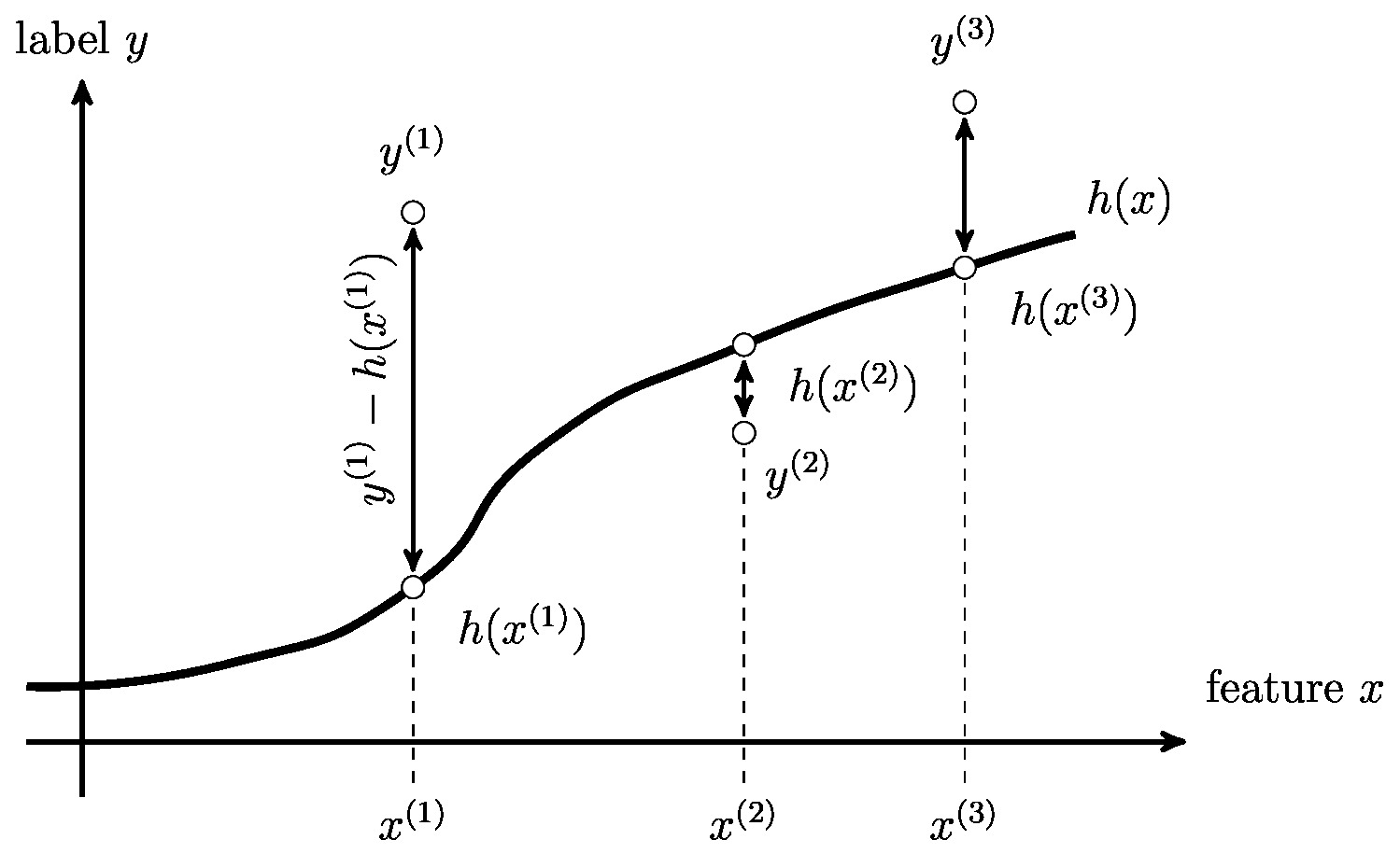
Notes
General References

Jung, Alexander (2022). Machine Learning: The Basics. Signapore: Springer. doi:10.1007/978-981-16-8193-6.
Jung, Alexander (2022). "Machine Learning: The Basics". arXiv:1805.05052.
References
- 1.0 1.1 F. Pedregosa. Scikit-learn: Machine learning in python. Journal of Machine Learning Research 12(85):2825--2830, 2011
- 2.0 2.1 D. Gujarati and D. Porter. Basic Econometrics Mc-Graw Hill, 2009
- 3.0 3.1 Y. Dodge. The Oxford Dictionary of Statistical Terms Oxford University Press, 2003
- 4.0 4.1 B. Everitt. Cambridge Dictionary of Statistics Cambridge University Press, 2002
- K. Abayomi, A. Gelman, and M. A. Levy. Diagnostics for multivariate imputations. Journal of The Royal Statistical Society Series C-applied Statistics 57:273--291, 2008
- M. Friendly. A brief history of data visualization. In C. Chen, W. Härdle, and A. Unwin, editors, Handbook of Computational Statistics: Data Visualization volume III. Springer-Verlag, 2006
- B. Boashash, editor. Time Frequency Signal Analysis and Processing: A Comprehensive Reference Elsevier, Amsterdam, The Netherlands, 2003
- S. G. Mallat. A Wavelet Tour of Signal Processing -- The Sparse Way Academic Press, San Diego, CA, 3 edition, 2009
- 9.0 9.1 W. Rudin. Principles of Mathematical Analysis McGraw-Hill, New York, 3 edition, 1976
- P. Bühlmann and S. van de Geer. Statistics for High-Dimensional Data Springer, New York, 2011
- M. Wainwright. High-Dimensional Statistics: A Non-Asymptotic Viewpoint Cambridge: Cambridge University Press, 2019
- R. Vidal. Subspace clustering. IEEE Signal Processing Magazine 52, March 2011
- T. Kibble and F. Berkshire. Classical Mechanics Imperical College Press, 5 edition, 2011
- F. Barata, K. Kipfer, M. Weber, P. Tinschert, E. Fleisch, and T. Kowatsch. Towards device-agnostic mobile cough detection with convolutional neural networks. In 2019 IEEE International Conference on Healthcare Informatics (ICHI) pages 1--11, 2019
- S. Smoliski and K. Radtke. Spatial prediction of demersal fish diversity in the baltic sea: comparison of machine learning and regression-based techniques. ICES Journal of Marine Science 74(1):102--111, 2017
- S. Carrazza. Machine learning challenges in theoretical HEP. arXiv 2018
- M. Gao, H. Igata, A. Takeuchi, K. Sato, and Y. Ikegaya. Machine learning-based prediction of adverse drug effects: An example of seizure-inducing compounds. Journal of Pharmacological Sciences 133(2):70 -- 78, 2017
- K. Mortensen and T. Hughes. Comparing amazon's mechanical turk platform to conventional data collection methods in the health and medical research literature. J. Gen. Intern Med. 33(4):533--538, 2018
- A. Halevy, P. Norvig, and F. Pereira. The unreasonable effectiveness of data. IEEE Intelligent Systems March/April 2009
- P. Koehn. Europarl: A parallel corpus for statistical machine translation. In The 10th Machine Translation Summit, page 79--86., AAMT, Phuket, Thailand, 2005
- 21.0 21.1 21.2 21.3 E. L. Lehmann and G. Casella. Theory of Point Estimation Springer, New York, 2nd edition, 1998
- S. M. Kay. Fundamentals of Statistical Signal Processing: Estimation Theory Prentice Hall, Englewood Cliffs, NJ, 1993
- 23.0 23.1 D. Bertsekas and J. Tsitsiklis. Introduction to Probability Athena Scientific, 2 edition, 2008
- 24.0 24.1 24.2 P. Billingsley. Probability and Measure Wiley, New York, 3 edition, 1995
- 25.0 25.1 C. M. Bishop. Pattern Recognition and Machine Learning Springer, 2006
- H. Lütkepohl. New Introduction to Multiple Time Series Analysis Springer, New York, 2005
- B. Efron and R. Tibshirani. Improvements on cross-validation: The 632+ bootstrap method. Journal of the American Statistical Association 92(438):548--560, 1997
- P. Halmos. Naive set theory Springer-Verlag, 1974
- P. Austin, P. Kaski, and K. Kubjas. Tensor network complexity of multilinear maps. arXiv 2018
- I. Goodfellow, Y. Bengio, and A. Courville. Deep Learning MIT Press, 2016
- 31.0 31.1 V. N. Vapnik. The Nature of Statistical Learning Theory Springer, 1999
- 32.0 32.1 S. Shalev-Shwartz and S. Ben-David. Understanding Machine Learning -- from Theory to Algorithms Cambridge University Press, 2014
- 33.0 33.1 T. Hastie, R. Tibshirani, and J. Friedman. The Elements of Statistical Learning Springer Series in Statistics. Springer, New York, NY, USA, 2001
- S. Bubeck. Convex optimization. algorithms and complexity. In Foundations and Trends in Machine Learning volume 8. Now Publishers, 2015
- M. J. Wainwright and M. I. Jordan. Graphical Models, Exponential Families, and Variational Inference volume 1 of Foundations and Trends in Machine Learning Now Publishers, Hanover, MA, 2008
- R. Gray. Probability, Random Processes, and Ergodic Properties Springer, New York, 2 edition, 2009
- R. Baeza-Yates and B. Ribeiro-Neto. Modern Information Retrieval addwes, 1999
- M. Abramowitz and I. A. Stegun, editors. Handbook of Mathematical Functions Dover, New York, 1965
- 39.0 39.1 39.2 N. Cesa-Bianchi and G. Lugosi. Prediction, Learning, and Games Cambridge University Press, New York, NY, USA, 2006
- E. Hazan. Introduction to Online Convex Optimization Now Publishers Inc., 2016
- R. Sutton and A. Barto. Reinforcement learning: An introduction MIT press, Cambridge, MA, 2 edition, 2018
- S. Boyd and L. Vandenberghe. Convex Optimization Cambridge Univ. Press, Cambridge, UK, 2004
