guide:013ef4b5cd

[math] \( % Generic syms \newcommand\defeq{:=} \newcommand{\Tt}[0]{\boldsymbol{\theta}} \newcommand{\XX}[0]{{\cal X}} \newcommand{\ZZ}[0]{{\cal Z}} \newcommand{\vx}[0]{{\bf x}} \newcommand{\vv}[0]{{\bf v}} \newcommand{\vu}[0]{{\bf u}} \newcommand{\vs}[0]{{\bf s}} \newcommand{\vm}[0]{{\bf m}} \newcommand{\vq}[0]{{\bf q}} \newcommand{\mX}[0]{{\bf X}} \newcommand{\mC}[0]{{\bf C}} \newcommand{\mA}[0]{{\bf A}} \newcommand{\mL}[0]{{\bf L}} \newcommand{\fscore}[0]{F_{1}} \newcommand{\sparsity}{s} \newcommand{\mW}[0]{{\bf W}} \newcommand{\mD}[0]{{\bf D}} \newcommand{\mZ}[0]{{\bf Z}} \newcommand{\vw}[0]{{\bf w}} \newcommand{\D}[0]{{\mathcal{D}}} \newcommand{\mP}{\mathbf{P}} \newcommand{\mQ}{\mathbf{Q}} \newcommand{\E}[0]{{\mathbb{E}}} \newcommand{\vy}[0]{{\bf y}} \newcommand{\va}[0]{{\bf a}} \newcommand{\vn}[0]{{\bf n}} \newcommand{\vb}[0]{{\bf b}} \newcommand{\vr}[0]{{\bf r}} \newcommand{\vz}[0]{{\bf z}} \newcommand{\N}[0]{{\mathcal{N}}} \newcommand{\vc}[0]{{\bf c}} \newcommand{\bm}{\boldsymbol} % Statistics and Probability Theory \newcommand{\errprob}{p_{\rm err}} \newcommand{\prob}[1]{p({#1})} \newcommand{\pdf}[1]{p({#1})} \def \expect {\mathbb{E} } % Machine Learning Symbols \newcommand{\biasterm}{B} \newcommand{\varianceterm}{V} \newcommand{\neighbourhood}[1]{\mathcal{N}^{(#1)}} \newcommand{\nrfolds}{k} \newcommand{\mseesterr}{E_{\rm est}} \newcommand{\bootstrapidx}{b} %\newcommand{\modeldim}{r} \newcommand{\modelidx}{l} \newcommand{\nrbootstraps}{B} \newcommand{\sampleweight}[1]{q^{(#1)}} \newcommand{\nrcategories}{K} \newcommand{\splitratio}[0]{{\rho}} \newcommand{\norm}[1]{\Vert {#1} \Vert} \newcommand{\sqeuclnorm}[1]{\big\Vert {#1} \big\Vert^{2}_{2}} \newcommand{\bmx}[0]{\begin{bmatrix}} \newcommand{\emx}[0]{\end{bmatrix}} \newcommand{\T}[0]{\text{T}} \DeclareMathOperator*{\rank}{rank} %\newcommand\defeq{:=} \newcommand\eigvecS{\hat{\mathbf{u}}} \newcommand\eigvecCov{\mathbf{u}} \newcommand\eigvecCoventry{u} \newcommand{\featuredim}{n} \newcommand{\featurelenraw}{\featuredim'} \newcommand{\featurelen}{\featuredim} \newcommand{\samplingset}{\mathcal{M}} \newcommand{\samplesize}{m} \newcommand{\sampleidx}{i} \newcommand{\nractions}{A} \newcommand{\datapoint}{\vz} \newcommand{\actionidx}{a} \newcommand{\clusteridx}{c} \newcommand{\sizehypospace}{D} \newcommand{\nrcluster}{k} \newcommand{\nrseeds}{s} \newcommand{\featureidx}{j} \newcommand{\clustermean}{{\bm \mu}} \newcommand{\clustercov}{{\bm \Sigma}} \newcommand{\target}{y} \newcommand{\error}{E} \newcommand{\augidx}{b} \newcommand{\task}{\mathcal{T}} \newcommand{\nrtasks}{T} \newcommand{\taskidx}{t} \newcommand\truelabel{y} \newcommand{\polydegree}{r} \newcommand\labelvec{\vy} \newcommand\featurevec{\vx} \newcommand\feature{x} \newcommand\predictedlabel{\hat{y}} \newcommand\dataset{\mathcal{D}} \newcommand\trainset{\dataset^{(\rm train)}} \newcommand\valset{\dataset^{(\rm val)}} \newcommand\realcoorspace[1]{\mathbb{R}^{\text{#1}}} \newcommand\effdim[1]{d_{\rm eff} \left( #1 \right)} \newcommand{\inspace}{\mathcal{X}} \newcommand{\sigmoid}{\sigma} \newcommand{\outspace}{\mathcal{Y}} \newcommand{\hypospace}{\mathcal{H}} \newcommand{\emperror}{\widehat{L}} \newcommand\risk[1]{\expect \big \{ \loss{(\featurevec,\truelabel)}{#1} \big\}} \newcommand{\featurespace}{\mathcal{X}} \newcommand{\labelspace}{\mathcal{Y}} \newcommand{\rawfeaturevec}{\mathbf{z}} \newcommand{\rawfeature}{z} \newcommand{\condent}{H} \newcommand{\explanation}{e} \newcommand{\explainset}{\mathcal{E}} \newcommand{\user}{u} \newcommand{\actfun}{\sigma} \newcommand{\noisygrad}{g} \newcommand{\reconstrmap}{r} \newcommand{\predictor}{h} \newcommand{\eigval}[1]{\lambda_{#1}} \newcommand{\regparam}{\lambda} \newcommand{\lrate}{\alpha} \newcommand{\edges}{\mathcal{E}} \newcommand{\generror}{E} \DeclareMathOperator{\supp}{supp} %\newcommand{\loss}[3]{L({#1},{#2},{#3})} \newcommand{\loss}[2]{L\big({#1},{#2}\big)} \newcommand{\clusterspread}[2]{L^{2}_{\clusteridx}\big({#1},{#2}\big)} \newcommand{\determinant}[1]{{\rm det}({#1})} \DeclareMathOperator*{\argmax}{argmax} \DeclareMathOperator*{\argmin}{argmin} \newcommand{\itercntr}{r} \newcommand{\state}{s} \newcommand{\statespace}{\mathcal{S}} \newcommand{\timeidx}{t} \newcommand{\optpolicy}{\pi_{*}} \newcommand{\appoptpolicy}{\hat{\pi}} \newcommand{\dummyidx}{j} \newcommand{\gridsizex}{K} \newcommand{\gridsizey}{L} \newcommand{\localdataset}{\mathcal{X}} \newcommand{\reward}{r} \newcommand{\cumreward}{G} \newcommand{\return}{\cumreward} \newcommand{\action}{a} \newcommand\actionset{\mathcal{A}} \newcommand{\obstacles}{\mathcal{B}} \newcommand{\valuefunc}[1]{v_{#1}} \newcommand{\gridcell}[2]{\langle #1, #2 \rangle} \newcommand{\pair}[2]{\langle #1, #2 \rangle} \newcommand{\mdp}[5]{\langle #1, #2, #3, #4, #5 \rangle} \newcommand{\actionvalue}[1]{q_{#1}} \newcommand{\transition}{\mathcal{T}} \newcommand{\policy}{\pi} \newcommand{\charger}{c} \newcommand{\itervar}{k} \newcommand{\discount}{\gamma} \newcommand{\rumba}{Rumba} \newcommand{\actionnorth}{\rm N} \newcommand{\actionsouth}{\rm S} \newcommand{\actioneast}{\rm E} \newcommand{\actionwest}{\rm W} \newcommand{\chargingstations}{\mathcal{C}} \newcommand{\basisfunc}{\phi} \newcommand{\augparam}{B} \newcommand{\valerror}{E_{v}} \newcommand{\trainerror}{E_{t}} \newcommand{\foldidx}{b} \newcommand{\testset}{\dataset^{(\rm test)} } \newcommand{\testerror}{E^{(\rm test)}} \newcommand{\nrmodels}{M} \newcommand{\benchmarkerror}{E^{(\rm ref)}} \newcommand{\lossfun}{L} \newcommand{\datacluster}[1]{\mathcal{C}^{(#1)}} \newcommand{\cluster}{\mathcal{C}} \newcommand{\bayeshypothesis}{h^{*}} \newcommand{\featuremtx}{\mX} \newcommand{\weight}{w} \newcommand{\weights}{\vw} \newcommand{\regularizer}{\mathcal{R}} \newcommand{\decreg}[1]{\mathcal{R}_{#1}} \newcommand{\naturalnumbers}{\mathbb{N}} \newcommand{\featuremapvec}{{\bf \Phi}} \newcommand{\featuremap}{\phi} \newcommand{\batchsize}{B} \newcommand{\batch}{\mathcal{B}} \newcommand{\foldsize}{B} \newcommand{\nriter}{R} [/math]

File:Fig ML methods loss hypo 2d

ML methods fit a model to data by minimizing a loss function. Different ML methods use different design choices for data, model and loss.

As discussed in Chapter Three Components of ML , ML methods combine three main components:

• a set of data points that are characterized by features and labels
• a model or hypothesis space[math]\hypospace[/math] that consists of different hypotheses [math]h \in \hypospace[/math].
• a loss function to measure the quality of a particular hypothesis [math]h[/math].

Each of these three components involves design choices for the representation of data, their features and labels, the model and loss function. This chapter details the high-level design choices used by some of the most popular ML methods.

Figure fig_ML_methods_loss_hypo_2d depicts these ML methods in a two-dimensional plane whose horizontal axes represents different hypothesis spaces and the vertical axis represents different loss functions.

To obtain a practical ML method we also need to combine the above components. The basic principle of any ML method is to search the model for a hypothesis that incurs minimum loss on any data point. Chapter Empirical Risk Minimization will then discuss a principled way to turn this informal statement into actual ML algorithms that could be implemented on a computer.

Linear Regression

Consider data points characterized by feature vectors [math]\featurevec \in \mathbb{R}^{\featuredim}[/math] and numeric label [math]\truelabel \in \mathbb{R}[/math]. Linear regression methods learn a hypothesis out of the linear hypothesis space

[[math]] \begin{align} \label{equ_lin_hypospace} \hypospace^{(\featuredim)} & \defeq \{ h^{(\weights)}: \mathbb{R}^{\featuredim}\!\rightarrow\!\mathbb{R}: h^{(\weights)}(\featurevec)\!=\!\weights^{T} \featurevec \mbox{ with some parameter vector } \weights \in \mathbb{R}^{\featuredim} \}. \end{align} [[/math]]

Figure fig_three_maps_example depicts the graphs of some maps from [math]\hypospace^{(2)}[/math] for data points with feature vectors of the form [math]\featurevec = (1,\feature)^{T}[/math]. The quality of a particular predictor [math]h^{(\weights)}[/math] is measured by the squared error loss. Using labeled data [math]\dataset =\{ (\featurevec^{(\sampleidx)},\truelabel^{(\sampleidx)}) \}_{\sampleidx=1}^{\samplesize}[/math], linear regression learns a linear predictor [math]\hat{h}[/math] which minimizes the average squared error loss squared error loss, or “mean squared error”,

[[math]] \begin{align} \label{equ_opt_pred_linreg} \hat{h} & = \argmin_{h \in \hypospace^{(\featuredim)} }\emperror(h|\dataset) \stackrel{\eqref{eq_def_emp_error_101}}{=} \argmin_{h \in \hypospace^{(\featuredim)} } (1/\samplesize) \sum_{\sampleidx=1}^{\samplesize} (\truelabel^{(\sampleidx)} - h(\featurevec^{(\sampleidx)}))^{2}. \end{align} [[/math]]

Since the hypothesis space [math]\hypospace^{(\featuredim)} [/math] is parametrized by the parameter vector [math]\weights[/math] (see \eqref{equ_lin_hypospace}), we can rewrite \eqref{equ_opt_pred_linreg} as an optimization of the parameter vector [math]\weights[/math],

[[math]] \begin{align} \widehat{\weights} & = \argmin_{\weights \in \mathbb{R}^{\featuredim}} (1/\samplesize) \sum_{\sampleidx=1}^{\samplesize} (\truelabel^{(\sampleidx)} - h^{(\weights)}(\featurevec^{(\sampleidx)}))^{2} \nonumber \\ & \label{equ_opt_weight_vector_linreg_weight}\stackrel{h^{(\weights)}(\featurevec) = \weights^{T} \featurevec}{=} \argmin_{\weights \in \mathbb{R}^{\featuredim}} (1/\samplesize) \sum_{\sampleidx=1}^{\samplesize} (\truelabel^{(\sampleidx)} - \weights^{T} \featurevec^{(\sampleidx)})^{2}. \end{align} [[/math]]

The optimization problems \eqref{equ_opt_pred_linreg} and \eqref{equ_opt_weight_vector_linreg_weight} are equivalent in the following sense: Any optimal parameter vector [math]\widehat{\weights}[/math] which solves \eqref{equ_opt_weight_vector_linreg_weight}, can be used to construct an optimal predictor [math]\hat{h}[/math], which solves \eqref{equ_opt_pred_linreg}, via [math]\hat{h}(\featurevec) = h^{(\widehat{\weights})}(\featurevec) = \big(\widehat{\weights}\big)^{T} \featurevec[/math].

Polynomial Regression

Consider an ML problem involving data points which are characterized by a single numeric feature [math]\feature \in \mathbb{R}[/math] (the feature space is [math]\featurespace= \mathbb{R}[/math]) and a numeric label [math]\truelabel \in \mathbb{R}[/math] (the label space is [math]\labelspace= \mathbb{R}[/math]). We observe a bunch of labeled data points which are depicted in Figure fig_scatterplot_poly.

A scatterplot that depicts a set of data points [math](\feature^{(1)},\truelabel^{(1)}),\ldots,(\feature^{(\samplesize)},\truelabel^{(\samplesize)})[/math]. The [math]\sampleidx[/math]th data point is depicted by a dot whose coordinates are the feature [math]\feature^{(\sampleidx)}[/math] and label [math]\truelabel^{(\sampleidx)}[/math] of that data point.

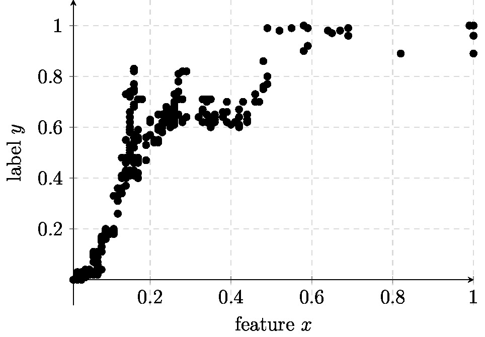
Figure fig_scatterplot_poly suggests that the relation [math]\feature \mapsto \truelabel[/math] between feature [math]\feature[/math] and label [math]\truelabel[/math] is highly non-linear. For such non-linear relations between features and labels it is useful to consider a hypothesis space which is constituted by polynomial maps

[[math]] \begin{align} \label{equ_def_poly_hyposapce} \hypospace^{(\featuredim)}_{\rm poly}& = \{ h^{(\weights)}: \mathbb{R} \rightarrow \mathbb{R}: h^{(\weights)}(\feature) = \sum_{\featureidx=1}^{\featuredim} \weight_{\featureidx} \feature^{\featureidx-1}, \nonumber \\  & \mbox{with some } \weights\!=\!(\weight_{1},\ldots,\weight_{\featuredim})^{T}\!\in\!\mathbb{R}^{\featuredim} \}. \end{align} [[/math]]

We can approximate any non-linear relation [math]\truelabel\!=\!h(\feature)[/math] with any desired level of accuracy using a polynomial [math]\sum_{\featureidx=1}^{\featuredim} \weight_{\featureidx} \feature^{\featureidx-1}[/math] of sufficiently large degree [math]\featuredim[/math].

For linear regression (see Section Linear Regression ), we measure the quality of a predictor by the squared error loss squared error loss. Based on labeled data points [math]\dataset =\{ (\feature^{(\sampleidx)},\truelabel^{(\sampleidx)}) \}_{\sampleidx=1}^{\samplesize}[/math], each having a scalar feature [math]\feature^{(\sampleidx)}[/math] and label [math]\truelabel^{(\sampleidx)}[/math], polynomial regression minimizes the average squared error loss (see squared error loss):

[[math]]\begin{equation} \label{opt_hypo_poly} \min_{h \in \hypospace_{\rm poly}^{(\featuredim)} } (1/\samplesize) \sum_{\sampleidx=1}^{\samplesize} (\truelabel^{(\sampleidx)} - h^{(\weights)}(\feature^{(\sampleidx)}))^{2}. \end{equation}[[/math]]

It is customary to refer to the average squared error loss also as the mean squared error.

We can interpret polynomial regression as a combination of a feature map (transformation) (see Section \ref{sec_feature_space}) and linear regression (see Section Linear Regression ). Indeed, any polynomial predictor [math]h^{(\weights)} \in \hypospace_{\rm poly}^{(\featuredim)}[/math] is obtained as a concatenation of the feature map

[[math]]\begin{equation} \label{equ_poly_feature_map} \featuremap(\feature) \mapsto (1,\feature,\ldots,\feature^{\featuredim})^{T} \in \mathbb{R}^{\featuredim+1} \end{equation}[[/math]]

with some linear map [math]\tilde{h}^{(\weights)}: \mathbb{R}^{\featuredim+1} \rightarrow \mathbb{R}: \featurevec \mapsto \weights^{T} \featurevec[/math], i.e.,

[[math]]\begin{equation} \label{equ_concact_phi_g_poly} h^{(\weights)}(\feature) = \tilde{h}^{(\weights)}(\featuremap(\feature)). \end{equation}[[/math]]

Thus, we can implement polynomial regression by first applying the feature map [math]\featuremap[/math] (see \eqref{equ_poly_feature_map}) to the scalar features [math]\feature^{(\sampleidx)}[/math], resulting in the transformed feature vectors

[[math]]\begin{equation} \label{equ_def_poly_feature_vectors} \featurevec^{(\sampleidx)} = \featuremap \big(\feature^{(\sampleidx)}\big) = \big(1,\feature^{(\sampleidx)},\ldots,\big( \feature^{(\sampleidx)} \big)^{\featuredim-1} \big)^{T} \in \mathbb{R}^{\featuredim}, \end{equation}[[/math]]

and then applying linear regression (see Section Linear Regression ) to these new feature vectors.

By inserting \eqref{equ_concact_phi_g_poly} into \eqref{opt_hypo_poly}, we obtain a linear regression problem \eqref{equ_opt_weight_vector_linreg_weight} with feature vectors \eqref{equ_def_poly_feature_vectors}. Thus, while a predictor [math]h^{(\vw)} \in \hypospace_{\rm poly}^{(\featuredim)}[/math] is a non-linear function [math]h^{(\vw)}(\feature)[/math] of the original feature [math]\feature[/math], it is a linear function [math]\tilde{h}^{(\weights)}(\featurevec) = \weights^{T}\featurevec[/math] (see \eqref{equ_concact_phi_g_poly}), of the transformed features [math]\featurevec[/math] \eqref{equ_def_poly_feature_vectors}.

Least Absolute Deviation Regression

Learning a linear predictor by minimizing the average squared error loss incurred on training data is not robust against the presence of outliers. This sensitivity to outliers is rooted in the properties of the squared error loss [math](\truelabel - h(\featurevec))^{2}[/math]. Minimizing the average squared error forces the resulting predictor [math]\hat{\truelabel}[/math] to not be too far away from any data point. However, it might be useful to tolerate a large prediction error [math]\truelabel - h ( \featurevec)[/math] for an unusual or exceptional data point that can be considered an outlier.

Replacing the squared loss with a different loss function can make the learning robust against outliers. One important example for such a “robustifying” loss function is the Huber loss

[[math]]\begin{equation} \label{equ_def_Huber_loss} \loss{\big(\featurevec,\truelabel \big)}{h} = \begin{cases} (1/2) (\truelabel-h(\featurevec))^{2} & \mbox{ for } |\truelabel-h(\featurevec)| \leq \varepsilon \\ \varepsilon(|\truelabel-h(\featurevec)| - \varepsilon/2) & \mbox{ else. }\end{cases} \end{equation}[[/math]]

Figure fig_Huber_loss depicts the Huber loss as a function of the prediction error [math]\truelabel - h(\featurevec)[/math].

The Huber loss \eqref{equ_def_Huber_loss} resembles the squared error loss

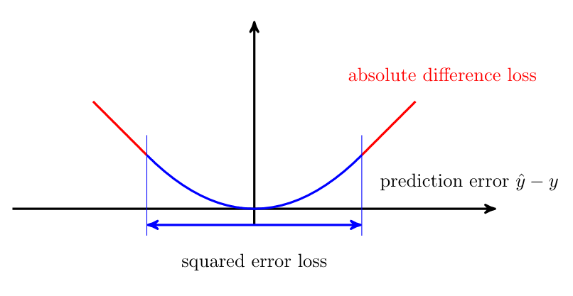
The Huber loss definition \eqref{equ_def_Huber_loss} contains a tuning parameter [math]\epsilon[/math]. The value of this tuning parameter defines when a data point is considered as an outlier. Figure fig_huber_loss_scatter illustrates the role of this parameter as the width of a band around a hypothesis map. The prediction error of this hypothesis map for data points within this band are measured used squared error loss. For data points outside this band (outliers) we use instead the absolute value of the prediction error as the resulting loss.

The Huber loss measures prediction errors via squared error loss for regular data points inside the band of width [math]\varepsilon[/math] around the hypothesis map [math]h(\featurevec)[/math] and via the absolute difference loss for an outlier outside the band.

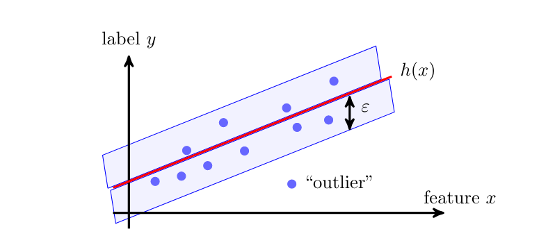
The Huber loss is robust to outliers since the corresponding (large) prediction errors [math]\truelabel - \hat{\truelabel}[/math] are not squared. Outliers have a smaller effect on the average Huber loss (over the entire dataset) compared to the average squared error loss. The improved robustness against outliers of the Huber loss comes at the expense of increased computational complexity. The squared error loss can be minimized using efficient gradient based methods (see Chapter Gradient-Based Learning ). In contrast, for [math]\varepsilon=0[/math], the Huber loss is non-differentiable and requires more advanced optimization methods.

The Huber loss \eqref{equ_def_Huber_loss} contains two important special cases. The first special case occurs when [math]\varepsilon[/math] is chosen to be very large, such that the condition [math]|\truelabel-\hat{\truelabel}| \leq \varepsilon[/math] is satisfied for most data points. In this case, the Huber loss resembles the squared error loss squared error loss (up to a scaling factor [math]1/2[/math]). The second special case is obtained for [math]\varepsilon=0[/math]. Here, the Huber loss reduces to the scaled absolute difference loss [math]|\truelabel - \hat{\truelabel}|[/math].

The Lasso

We will see in Chapter Model Validation and Selection that linear regression (see Section Linear Regression ) typically requires a training set larger than the number of features used to characterized a data point. However, many important application domains generate data points with a number [math]\featuredim[/math] of features much higher than the number [math]\samplesize[/math] of available labeled data points in the training set.

In the high-dimensional regime, where [math]\samplesize \ll \featurelen[/math], basic linear regression methods will not be able to learn useful weights [math]\weights[/math] for a linear hypothesis. Section A Probabilistic Analysis of Generalization shows that for [math]\samplesize \ll \featurelen[/math], linear regression will typically learn a hypothesis that perfectly predicts labels of data points in the training set but delivers poor predictions for data points outside the training set. This phenomenon is referred to as overfitting and poses a main challenge for ML applications in the high-dimensional regime.

Chapter Regularization discusses basic regularization techniques that allow to prevent ML methods from overfitting. We can regularize linear regression by augmenting the squared error loss squared error loss of a hypothesis [math]h^{(\weights)}(\featurevec) = \weights^{T} \featurevec[/math] with an additional penalty term. This penalty term depends solely on the weights [math]\weights[/math] and serves as an estimate for the increase of the average loss on data points outside the training set. Different ML methods are obtained from different choices for this penalty term. The least absolute shrinkage and selection operator (Lasso) is obtained from linear regression by replacing the squared error loss with the regularized loss

[[math]]\begin{equation}\label{equ_def_reg_loss_lin_reg} \loss{(\featurevec,\truelabel)}{h^{(\vw)}} = (\truelabel-\weights^{T}\featurevec)^{2} + \regparam \| \weights \|_{1}. \end{equation}[[/math]]

Here, the penalty term is given by the scaled norm [math]\regparam \| \vw \|_{1}[/math]. The value of [math]\regparam[/math] can be chosen based on some probabilistic model that interprets a data point as the realization of a random variable (RV). The label of this data point (which is a realization of a RV) is related to its features via

[[math]]\truelabel = \overline{\weights}^{T} \featurevec + \varepsilon.[[/math]]

Here, [math]\overline{\weights}[/math] denotes some true underlying parameter vector and [math]\varepsilon[/math] is a realization of an a RV that is independent of the features [math]\featurevec[/math]. We need the “noise” term [math]\varepsilon[/math] since the labels of data points collected in some ML application are typically not exactly obtained by a linear combination [math]\overline{\weights}^{T} \featurevec[/math] of its features.

The tuning of [math]\regparam[/math] in \eqref{equ_def_reg_loss_lin_reg} can be guided by the statistical properties (such as the variance) of the noise [math]\varepsilon[/math], the number of non-zero entries in [math]\overline{\weights}[/math] and a lower bound on the non-zero values . Another option for choosing the value [math]\regparam[/math] is to try out different candidate values and pick the one resulting in smallest validation error (see Section Validation ).

Gaussian Basis Regression

Section Polynomial Regression showed how to extend linear regression by first transforming the feature [math]\feature[/math] using a vector-valued feature map [math]\featuremap: \mathbb{R} \rightarrow \mathbb{R}^{\featuredim}[/math]. The output of this feature map are the transformed features [math]\featuremap(\feature)[/math] which are fed, in turn, to a linear map [math]h\big(\featuremap(\feature)\big) = \weights^{T} \featuremap(\feature)[/math]. Polynomial regression in Section Polynomial Regression has been obtained for the specific feature map \eqref{equ_poly_feature_map} whose entries are the powers [math]\feature^{l}[/math] of the scalar original feature [math]\feature[/math]. However, it is possible to use other functions, different from polynomials, to construct the feature map [math]\featuremap[/math]. We can extend linear regression using an arbitrary feature map

[[math]]\begin{equation} \featuremap(\feature) = (\basisfunc_{1}(\feature),\ldots,\basisfunc_{\featuredim}(\feature))^{T} \end{equation}[[/math]]

with the scalar maps [math]\basisfunc_{\featureidx}: \mathbb{R} \rightarrow \mathbb{R}[/math] which are referred to as “basis functions”. The choice of basis functions depends heavily on the particular application and the underlying relation between features and labels of the observed data points. The basis functions underlying polynomial regression are [math]\basisfunc_{\featureidx}(\feature)= \feature^{\featureidx}[/math].

Another popular choice for the basis functions are “Gaussians”

[[math]]\begin{equation} \label{equ_basis_Gaussian} \phi_{\sigma,\mu}(\feature) = \exp(-(1/(2\sigma^{2})) (\feature\!-\!\mu)^{2}). \end{equation}[[/math]]

The family \eqref{equ_basis_Gaussian} of maps is parameterized by the variance [math]\sigma^{2}[/math] and the mean (shift) [math]\mu[/math]. Gaussian basis linear regression combines the feature map

[[math]]\begin{equation} \featuremap(\feature) = \big (\phi_{\sigma_{1},\mu_{1}}(\feature) ,\ldots,\phi_{\sigma_{\featuredim},\mu_{\featuredim}}(\feature) \big)^{T} \end{equation}[[/math]]

with linear regression (see Figure fig_lin_bas_expansion). The resulting hypothesis space is

[[math]] \begin{align} \hypospace^{(\featuredim)}_{\rm Gauss} & = \{ h^{(\weights)}: \mathbb{R} \rightarrow \mathbb{R}: h^{(\weights)}(\feature)\!=\!\sum_{\featureidx=1}^{\featuredim} \weight_{\featureidx}\phi_{\sigma_{\featureidx},\mu_{\featureidx}}(\feature) \nonumber \\ & \label{equ_def_Gauss_hypospace}\mbox{ with weights } \weights=(\weight_{1},\ldots,\weight_{\featuredim})^{T} \in \mathbb{R}^{\featuredim}\}. \end{align} [[/math]]

Different choices for the variance [math]\sigma_{\featureidx}^{2}[/math] and shifts [math]\mu_{\featureidx}[/math] of the Gaussian function in \eqref{equ_basis_Gaussian} results in different hypothesis spaces [math]\hypospace_{\rm Gauss}[/math]. Chapter Model Selection will discuss model selection techniques that allow to find useful values for these parameters.

The hypotheses of \eqref{equ_def_Gauss_hypospace} are parametrized by a parameter vector [math]\weights \in \mathbb{R}^{\featuredim}[/math]. Each hypothesis in [math]\hypospace_{\rm Gauss}[/math] corresponds to a particular choice for the parameter vector [math]\weights[/math]. Thus, instead of searching over [math]\hypospace_{\rm Gauss}[/math] to find a good hypothesis, we can search over the Euclidean space [math]\mathbb{R}^{\featuredim}[/math]. Highly developed methods for searching over the space [math]\mathbb{R}^{\featuredim}[/math], for a wide range of values for [math]\featuredim[/math], are provided by numerical linear algebra .

The true relation [math]\feature \mapsto \truelabel[/math] (blue) between feature [math]\feature[/math] and label [math]\truelabel[/math] of data points is highly non-linear. Therefore it seems reasonable to predict the label using a non-linear hypothesis map [math]h^{(\weights)}(\feature) \!\in\!\hypospace^{(2)}_{\rm Gauss}[/math] with some parameter vector [math]\weights \in \mathbb{R}^{2}[/math].

Logistic Regression

Logistic regression is a ML method that allows to classify data points according to two categories. Thus, logistic regression is a binary classification method that can be applied to data points characterized by feature vectors [math]\featurevec \in \mathbb{R}^{\featuredim}[/math] (feature space [math]\featurespace=\mathbb{R}^{\featuredim}[/math]) and binary labels [math]\truelabel[/math]. These binary labels take on values from a label space that contains two different label values. Each of these two label values represents one of the two categories to which the data points can belong.

It is convenient to use the label space [math]\labelspace = \mathbb{R}[/math] and encode the two label values as [math]\truelabel=1[/math] and [math]\truelabel=-1[/math]. However, it is important to note that logistic regression can be used with an arbitrary label space which contains two different elements. Another popular choice for the label space is [math]\labelspace=\{0,1\}[/math]. Logistic regression learns a hypothesis out of the hypothesis space [math]\hypospace^{(\featuredim)}[/math] (see \eqref{equ_lin_hypospace}). Note that logistic regression uses the same hypothesis space as linear regression (see Section Linear Regression ).

At first sight, it seems wasteful to use a linear hypothesis [math]h(\featurevec) = \weights^T \featurevec[/math], with some parameter vector [math]\weights \in \mathbb{R}^{\featuredim}[/math], to predict a binary label [math]\truelabel[/math]. Indeed, while the prediction [math]h(\featurevec)[/math] can take any real number, the label [math]\truelabel \in \{-1,1\}[/math] takes on only one of the two real numbers [math]1[/math] and [math]-1[/math].

It turns out that even for binary labels it is quite useful to use a hypothesis map [math]h[/math] which can take on arbitrary real numbers. We can always obtain a predicted label [math]\hat{\truelabel} \in \{-1,1\}[/math] by comparing hypothesis value [math]h(\featurevec)[/math] with a threshold. A data point with features [math]\featurevec[/math], is classified as [math]\hat{\truelabel}=1[/math] if [math]h(\featurevec)\geq 0[/math] and [math]\hat{\truelabel}=-1[/math] for [math]h(\featurevec)\lt 0[/math]. Thus, we use the sign of the predictor [math]h[/math] to determine the final prediction for the label. The absolute value [math]|h(\featurevec)|[/math] is then used to quantify the reliability of (or confidence in) the classification [math]\hat{\truelabel}[/math].

Consider two data points with feature vectors [math]\featurevec^{(1)}, \featurevec^{(2)}[/math] and a linear classifier map [math]h[/math] yielding the function values [math]h(\featurevec^{(1)}) = 1/10[/math] and [math]h(\featurevec^{(2)}) = 100[/math]. Whereas the predictions for both data points result in the same label predictions, i.e., [math]\hat{\truelabel}^{(1)}\!=\!\hat{\truelabel}^{(2)}\!=\!1[/math], the classification of the data point with feature vector [math]\featurevec^{(2)}[/math] seems to be much more reliable.

Logistic regression uses the logistic loss to assess the quality of a particular hypothesis [math]h^{(\weights)} \in \hypospace^{(\featuredim)}[/math]. In particular, given some labeled training set [math]\dataset =\{ \featurevec^{(\sampleidx)},\truelabel^{(\sampleidx)} \}_{\sampleidx=1}^{\samplesize}[/math], logistic regression tries to minimize the empirical risk (average logistic loss)

[[math]] \begin{align} \emperror ( \weights | \dataset ) & = (1/\samplesize) \sum_{\sampleidx=1}^{\samplesize} \log( 1+ \exp ( - \truelabel^{(\sampleidx)} h^{(\weights)}(\featurevec^{(\sampleidx)}))) \nonumber \\ & \label{equ_def_emp_risk_logreg}\stackrel{h^{(\weights)}(\featurevec)=\weights^{T} \featurevec}{=} (1/\samplesize) \sum_{\sampleidx=1}^{\samplesize} \log( 1+ \exp ( - \truelabel^{(\sampleidx)} \weights^{T} \featurevec^{(\sampleidx)})). \end{align} [[/math]]

Once we have found the optimal parameter vector [math]\widehat{\weights}[/math], which minimizes \eqref{equ_def_emp_risk_logreg}, we can classify any data point solely based on its features [math]\featurevec[/math]. Indeed, we just need to evaluate the hypothesis [math]h^{(\widehat{\weights})}[/math] for the features [math]\featurevec[/math] to obtain the predicted label

[[math]]\begin{equation} \label{equ_class_logreg} \hat{\truelabel} = \begin{cases} 1 & \mbox{ if } h^{(\widehat{\weights})}(\featurevec) \geq 0 \\ -1 & \mbox{ otherwise.} \end{cases} \end{equation}[[/math]]

Since [math]h^{(\widehat{\weights})}(\featurevec) = \big(\widehat{\weights}\big)^{T} \featurevec[/math] (see \eqref{equ_lin_hypospace}), the classifier \eqref{equ_class_logreg} amounts to testing whether [math]\big(\widehat{\weights}\big)^{T} \featurevec \geq 0[/math] or not.

The classifier \eqref{equ_class_logreg} partitions the feature space [math]\featurespace\!=\!\mathbb{R}^{\featuredim}[/math] into two half-spaces [math]\decreg{1}\!=\!\big\{ \featurevec: \big(\widehat{\weights}\big)^{T} \featurevec\!\geq\!0 \big\}[/math] and [math]\decreg{-1}\!=\!\big\{ \featurevec: \big(\widehat{\weights}\big)^{T} \featurevec\!\lt\!0 \big\}[/math] which are separated by the hyperplane [math]\big(\widehat{\weights}\big)^{T} \featurevec =0[/math] (see Figure fig_lin_dec_boundary). Any data point with features [math]\featurevec \in \decreg{1}[/math] ([math]\featurevec \in \decreg{-1}[/math]) is classified as [math]\hat{\truelabel}\!=\!1[/math] ([math]\hat{\truelabel}\!=\!-1[/math]).

Logistic regression can be interpreted as a statistical estimation method for a particular probabilistic model for the data points. This probabilistic model interprets the label [math]\truelabel \in \{-1,1\}[/math] of a data point as a RV with the probability distribution

[[math]] \begin{align} \prob{\truelabel=1;\weights}& = 1/(1 + \exp(- \weights^{T} \featurevec) ) \nonumber \\ & \label{equ_prob_model_logistic_model}\stackrel{h^{(\weights)}(\featurevec)\!=\!\weights^{T} \featurevec}{=} 1/(1 + \exp(- h^{(\weights)}(\featurevec))) ) . \end{align} [[/math]]

As the notation indicates, the probability \eqref{equ_prob_model_logistic_model} is parametrized by the parameter vector [math]\weights[/math] of the linear hypothesis [math]h^{(\weights)}(\featurevec)\!=\!\weights^{T} \featurevec[/math]. Given the probabilistic model \eqref{equ_prob_model_logistic_model}, we can interpret the classification \eqref{equ_class_logreg} as choosing [math]\hat{\truelabel}[/math] to maximize the probability [math]\prob{\truelabel=\hat{\truelabel};\weights}[/math].

Since [math]\prob{\truelabel=1} + \prob{\truelabel=-1}=1[/math],

[[math]] \begin{align} \prob{\truelabel=-1} & = 1 - \prob{\truelabel=1} \nonumber \\ & \stackrel{\eqref{equ_prob_model_logistic_model}}{=} 1 - 1/(1+ \exp(-\weights^{T} \featurevec)) \nonumber \\ & = \label{equ_prob_model_logistic_model_minus_1} 1/(1+ \exp(\weights^{T} \featurevec)). \end{align} [[/math]]

In practice we do not know the parameter vector in \eqref{equ_prob_model_logistic_model}. Rather, we have to estimate the parameter vector [math]\weights[/math] in \eqref{equ_prob_model_logistic_model} from observed data points. A principled approach to estimate the parameter vector is to maximize the probability (or likelihood) of actually obtaining the dataset [math]\dataset=\{ (\featurevec^{(\sampleidx)},\truelabel^{(\sampleidx)}) \}_{\sampleidx=1}^{\samplesize}[/math] as realizations of independent and identically distributed (iid) data points whose labels are distributed according to \eqref{equ_prob_model_logistic_model}. This yields the maximum likelihood estimator

[[math]] \begin{align} \widehat{\weights} & = \argmax_{\weights \in \mathbb{R}^{\featuredim}} \prob{ \{\truelabel^{(\sampleidx)}\}_{\sampleidx=1}^{\samplesize}} \nonumber \\ & \stackrel{\truelabel^{(\sampleidx)}\mbox{iid}}{=} \argmax_{\vw \in \mathbb{R}^{\featuredim}} \prod_{\sampleidx=1}^{\samplesize} \prob { \truelabel^{(\sampleidx)}}\nonumber \\ & \label{equ_deriv_prog_logreg}\stackrel{\eqref{equ_prob_model_logistic_model},\eqref{equ_prob_model_logistic_model_minus_1}}{=} \argmax_{\vw \in \mathbb{R}^{\featuredim}} \prod_{\sampleidx=1}^{\samplesize} 1/(1 + \exp(- \truelabel^{(\sampleidx)} \weights^{T} \featurevec^{(\sampleidx)}) ). \end{align} [[/math]]

Note that the last expression \eqref{equ_deriv_prog_logreg} is only valid if we encode the binary labels using the values [math]1[/math] and [math]-1[/math]. Using different label values results in a different expression.

Maximizing a positive function [math]f(\weights)\gt0[/math] is equivalent to maximizing [math]\log f(\weight)[/math],

[[math]]\argmax\limits_{\weights \in \mathbb{R}^{\featuredim}} f(\weights)\!=\!\argmax\limits_{\weights \in \mathbb{R}^{\featuredim}}\log f(\weights).[[/math]]

Therefore, \eqref{equ_deriv_prog_logreg} can be further developed as

[[math]] \begin{align} \widehat{\weights} & \stackrel{\eqref{equ_deriv_prog_logreg}}{=} \argmax_{\weights \in \mathbb{R}^{\featuredim}} \sum_{\sampleidx=1}^{\samplesize} - \log\big(1\!+\!\exp(- \truelabel^{(\sampleidx)} \weights^{T} \featurevec^{(\sampleidx)}) \big) \nonumber \\ & = \label{equ_deriv_prog_logreg_2}\argmin_{\weights \in \mathbb{R}^{\featuredim}} (1/\samplesize)\sum_{\sampleidx=1}^{\samplesize} \log\big(1\!+\!\exp(- \truelabel^{(\sampleidx)}\vw^{T} \featurevec^{(\sampleidx)}) \big). \end{align} [[/math]]

Comparing \eqref{equ_deriv_prog_logreg_2} with \eqref{equ_def_emp_risk_logreg} reveals that logistic regression is nothing but maximum likelihood estimation of the parameter vector [math]\weights[/math] in the probabilistic model \eqref{equ_prob_model_logistic_model}.

Support Vector Machines

Support vector machine (SVM)s are a family of ML methods for learning a hypothesis to predict a binary label [math]\truelabel[/math] of a data point based on its features [math]\featurevec[/math]. Without loss of generality we consider binary labels taking values in the label space [math]\labelspace = \{-1,1\}[/math]. A support vector machine (SVM) uses the linear hypothesis space \eqref{equ_lin_hypospace} which consists of linear maps [math]h(\featurevec) = \weights^{T} \featurevec[/math] with some parameter vector [math]\weights \in \mathbb{R}^{\featuredim}[/math]. Thus, the SVM uses the same hypothesis space as linear regression and logistic regression which we have discussed in Section Linear Regression and Section Logistic Regression , respectively. What sets the SVM apart from these other methods is the choice of loss function.

Different instances of a SVM are obtained by using different constructions for the features of a data point. Kernel SVMs use the concept of a kernel map to construct (typically high-dimensional) features (see Section Kernel Methods and ). In what follows, we assume the feature construction has been solved and we have access to a feature vector [math]\featurevec \in \mathbb{R}^{\featuredim}[/math] for each data point.

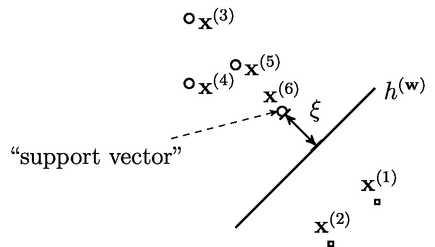
Figure fig_svm depicts a dataset [math]\dataset[/math] of labeled data points, each characterized by a feature vector [math]\featurevec^{(\sampleidx)} \in \mathbb{R}^{2}[/math] (used as coordinates of a marker) and a binary label [math]\truelabel^{(\sampleidx)} \in \{-1,1\}[/math] (indicated by different marker shapes). We can partition dataset [math]\dataset[/math] into two classes

[[math]]\begin{equation} \label{equ_two_classes_svm} \mathcal{C}^{(\truelabel=1)}\!=\!\{ \featurevec^{(\sampleidx)} : \truelabel^{(\sampleidx)}\!=\!1\}\mbox{, and }\mathcal{C}^{(\truelabel=-1)}\!=\!\{ \featurevec^{(\sampleidx)} : \truelabel^{(\sampleidx)}\!=\!-1 \}. \end{equation}[[/math]]

The SVM tries to learn a linear map [math]h^{(\weights)}(\featurevec) = \weights^{T} \featurevec[/math] that perfectly separates the two classes in the sense of

[[math]] \begin{align} \label{equ_two_classes_svm_perf_sep} \underbrace{h \big( \featurevec^{(\sampleidx)} \big)}_{\weights^{T} \featurevec^{(\sampleidx)} } \gt 0 \mbox{ for } \featurevec^{(\sampleidx)} \in \mathcal{C}^{(\truelabel=1)} \mbox{ and } \underbrace{h \big( \featurevec^{(\sampleidx)} \big)}_{\weights^{T} \featurevec^{(\sampleidx)} } \lt 0 \mbox{ for } \featurevec^{(\sampleidx)} \in \mathcal{C}^{(\truelabel=-1)}. \end{align} [[/math]]

We refer to a dataset, whose data points have binary labels. as linear separable if we can find at least one linear map that separates in the sense of \eqref{equ_two_classes_svm_perf_sep}. The dataset in Figure fig_svm is linearly separable.

As can be verified easily, any linear map [math]h^{(\weights)}(\featurevec) = \weights^{T} \featurevec[/math] achieving zero average hinge loss on the dataset [math]\dataset[/math] perfectly satisfies this dataset \eqref{equ_two_classes_svm_perf_sep}. It seems reasonable to learn a linear map by minimizing the average hinge loss. However, one drawback of this approach is that there might be (infinitely) many different linear maps that achieve zero average hinge loss and, in turn, perfectly separate the data points in Figure fig_svm. Indeed, consider a linear map [math]h^{(\weights)}[/math] that achieves zero average hinge loss for the [math]\dataset[/math] in Figure fig_svm (and therefore perfectly separates it). Then, any other linear map [math]h^{(\weights')}[/math] with weights [math]\weights' = \regparam \weights[/math], using an arbitrary number [math]\regparam \gt 1[/math] also achieves zero average hinge loss (and perfectly separates the dataset).

Neither the separability requirement \eqref{equ_two_classes_svm_perf_sep} nor the hinge loss are sufficient as a sole training criterion. Indeed, there are many (if not most) datasets that are not linearly separable. Even for a linearly separable dataset (such as the one Figure fig_svm), there are infinitely many linear maps with zero average hinge loss. Which one of these infinitely many different maps should we use? To settle these issues, the SVM uses a “regularized” hinge loss,

[[math]] \begin{align} \loss{(\featurevec,\truelabel)}{h^{(\weights)}} & \defeq \max \{ 0 , 1 - \truelabel\cdot h^{(\weights)}(\featurevec) \} + \regparam \sqeuclnorm{ \weights }\nonumber \\ & \stackrel{h^{(\weights)}(\featurevec) = \weights^{T} \featurevec}{=} \max \{ 0 , 1 - \truelabel\cdot \weights^{T} \featurevec \} + \regparam \sqeuclnorm{ \weights }. \label{equ_loss_svm} \end{align} [[/math]]

The loss \eqref{equ_loss_svm} augments the hinge loss by the term [math]\regparam \sqeuclnorm{\weights }[/math]. This term is the scaled (by [math]\regparam \gt0[/math]) squared Euclidean norm of the weights [math]\weights[/math] of the linear hypothesis [math]h[/math] used to classify data points. it can be shown that adding the term [math]\regparam \sqeuclnorm{ \weights }[/math] to the hinge loss has an regularization effect.

The loss \eqref{equ_loss_svm} favours linear maps [math]h^{(\weights)}[/math] that are robust against (small) perturbations of the data points. The tuning parameter [math]\regparam[/math] in \eqref{equ_loss_svm} controls the strength of this regularization effect and might therefore also be referred to as a regularization parameter. We will discuss regularization on a more general level in Chapter Regularization .

Let us now develop a useful geometric interpretation of the linear hypothesis obtained by minimizing the loss function \eqref{equ_loss_svm}. According to , a classifier [math]h^{(\weights_{\rm SVM})}[/math] that minimizes the average loss \eqref{equ_loss_svm}, maximizes the distance (margin) [math]\xi[/math] between its decision boundary and each of the two classes [math]\cluster^{(\truelabel=1)}[/math] and [math]\cluster^{(\truelabel=-1)}[/math] (see \eqref{equ_two_classes_svm}). The decision boundary is given by the set of feature vectors [math]\featurevec[/math] satisfying [math]\weights_{\rm SVM}^{T} \featurevec=0[/math],

Making the margin as large as possible is reasonable as it ensures that the resulting classifications are robust against small perturbations of the features (see Section Robustness ). As depicted in Figure fig_svm, the margin between the decision boundary and the classes [math]\mathcal{C}_{1}[/math] and [math]\mathcal{C}_{2}[/math] is typically determined by few data points (such as [math]\featurevec^{(6)}[/math] in Figure fig_svm) which are closest to the decision boundary. These data points have minimum distance to the decision boundary and are referred to as support vectors.

The SVM learns a hypothesis (or classifier) [math]h^{(\weights)}[/math] with minimum average soft-margin hinge loss \eqref{equ_loss_svm}. Minimizing this loss is equivalent to maximizing the margin [math]\xi[/math] between the decision boundary of [math]h^{(\weights)}[/math] and each class of the training set.

We highlight that both, the SVM and logistic regression use the same hypothesis space of linear maps. Both methods learn a linear classifier [math]h^{(\weights)} \in \hypospace^{(\featuredim)}[/math] (see \eqref{equ_lin_hypospace}) whose decision boundary is a hyperplane in the feature space [math]\featurespace = \mathbb{R}^{\featuredim}[/math] (see Figure fig_lin_dec_boundary). The difference between SVM and logistic regression is in their choice for the loss function used to evaluate the quality of a hypothesis [math]h^{(\weights)} \in \hypospace^{(\featuredim)}[/math].

The hinge loss is a (in some sense optimal) convex approximation to the 0/1 loss. Thus, we expect the classifier obtained by the SVM to yield a smaller classification error probability [math]\prob{ \predictedlabel \neq \truelabel }[/math] (with [math]\predictedlabel =1[/math] if [math]h(\featurevec)\geq0[/math] and [math]\predictedlabel=-1[/math] otherwise) compared to logistic regression which uses the logistic loss. The SVM is also statistically appealing as it learns a robust hypothesis. Indeed, the hypothesis map with maximum margin is maximally robust against perturbations of the feature vectors of data points. Section Robustness discusses the importance of robustness in ML methods in more detail.

The statistical superiority (in terms of robustness) of the SVM comes at the cost of increased computational complexity. The hinge loss is non-differentiable which prevents the use of simple gradient-based methods (see Chapter Gradient-Based Learning ) and requires more advanced optimization methods. In contrast, the logistic loss is convex and differentiable. Logistic regression allows for the use of gradient-based methods to minimize the average logistic loss incurred on a training set (see Chapter Gradient-Based Learning ).

Bayes Classifier

Consider data points characterized by features [math]\featurevec \in \featurespace[/math] and some binary label [math]\truelabel \in \labelspace[/math]. We can use any two different label values but let us assume that the two possible label values are [math]\truelabel=-1[/math] or [math]\truelabel=1[/math]. We would like to find (or learn) a classifier [math]h: \featurespace \rightarrow \labelspace[/math] such that the predicted (or estimated) label [math]\hat{\truelabel} = h(\featurevec)[/math] agrees with the true label [math]\truelabel \in \labelspace[/math] as much as possible. Thus, it is reasonable to assess the quality of a classifier [math]h[/math] using the 0/1 loss. We could then learn a classifier using the empirical risk minimization (ERM) with the 0/1 loss. However, the resulting optimization problem is typically intractable since the 0/1 loss is non-convex and non-differentiable.

Instead of solving the (intractable) ERM for 0/1 loss, we can take a different route to construct a classifier. This construction is based on a simple probabilistic model for data. Using this model, we can interpret the average [math]0/1[/math] loss incurred by a hypothesis on a training set as an approximation to the probability [math]\errprob = \prob{ \truelabel \neq h(\featurevec) }[/math]. Any classifier [math]\hat{h}[/math] that minimizes the error probability [math]\errprob[/math], which is the expected [math]0/1[/math] loss, is referred to as a Bayes estimator. Section ERM for Bayes Classifiers will discuss ML methods using Bayes estimator in more detail.

Let us derive the Bayes estimator for a the special case of a binary classification problem. Here, data points are characterized by features [math]\featurevec[/math] and label [math]\truelabel \in \{-1,1\}[/math]. Elementary probability theory allows to derive the Bayes estimator, which is the hypothesis minimizing the expected [math]0/1[/math] loss, as

[[math]]\begin{equation} \label{equ_def_Bayes_est_binary_class} \hat{h}(\featurevec) = \begin{cases} 1 & \mbox{ if } \prob{\truelabel = 1| \featurevec } \gt \prob{\truelabel = -1| \featurevec } \\ - 1 & \mbox{ otherwise.} \end{cases}. \end{equation}[[/math]]

Note that the Bayes estimator \eqref{equ_def_Bayes_est_binary_class} depends on the probability distribution [math]\prob{\featurevec,\truelabel}[/math] underlying the data points.\footnote{Remember that we interpret data points as realizations of iid RVs with common probability distribution [math]\prob{\featurevec,\truelabel}[/math].} We obtain different Bayes estimators for different probabilistic models. One widely used probabilistic model results in a Bayes estimator that belongs to the linear hypothesis space \eqref{equ_lin_hypospace}. Note that this hypothesis space underlies also logistic regression (see Section Logistic Regression ) and the SVM (see Section Support Vector Machines ). Thus, logistic regression, SVM and Bayes estimator are all examples of a linear classifier (see Figure fig_lin_dec_boundary).

A linear classifier partitions the feature space [math]\featurespace[/math] into two half-spaces. One half-space consists of all feature vectors [math]\featurevec[/math] which result in the predicted label [math]\predictedlabel=1[/math] and the other half-space constituted by all feature vectors [math]\featurevec[/math] which result in the predicted label [math]\predictedlabel=-1[/math]. The family of ML methods that learn a linear classifier differ in their choices for the loss functions used to assess the quality of these half-spaces.

Kernel Methods

Consider a ML (classification or regression) problem with an underlying feature space [math]\featurespace[/math]. In order to predict the label [math]y \in \labelspace[/math] of a data point based on its features [math]\featurevec \in \featurespace[/math], we apply a predictor [math]h[/math] selected out of some hypothesis space [math]\hypospace[/math]. Let us assume that the available computational infrastructure only allows us to use a linear hypothesis space [math]\hypospace^{(\featuredim)}[/math] (see \eqref{equ_lin_hypospace}).

For some applications, using a linear hypothesis [math]h(\featurevec)=\weights^{T}\featurevec[/math] is not suitable since the relation between features [math]\featurevec[/math] and label [math]\truelabel[/math] might be highly non-linear. One approach to extend the capabilities of linear hypotheses is to transform the raw features of a data point before applying a linear hypothesis [math]h[/math].

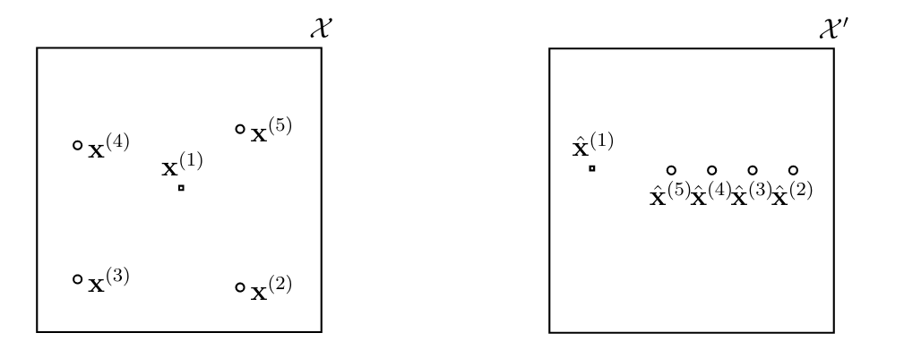
The family of kernel methods is based on transforming the features [math]\featurevec[/math] to new features [math]\hat{\featurevec} \in \featurespace'[/math] which belong to a (typically very) high-dimensional space [math]\featurespace'[/math] . It is not uncommon that, while the original feature space is a low-dimensional Euclidean space (e.g., [math]\featurespace = \mathbb{R}^{2}[/math]), the transformed feature space [math]\featurespace'[/math] is an infinite-dimensional function space.

The rationale behind transforming the original features into a new (higher-dimensional) feature space [math]\featurespace'[/math] is to reshape the intrinsic geometry of the feature vectors [math]\featurevec^{(\sampleidx)} \in \featurespace[/math] such that the transformed feature vectors [math]\hat{\featurevec}^{(\sampleidx)}[/math] have a “simpler” geometry (see Figure fig_kernelmethods).

Kernel methods are obtained by formulating ML problems (such as linear regression or logistic regression) using the transformed features [math]\hat{\featurevec}= \phi(\featurevec)[/math]. A key challenge within kernel methods is the choice of the feature map [math]\phi: \featurespace \rightarrow \featurespace'[/math] which maps the original feature vector [math]\featurevec[/math] to a new feature vector [math]\hat{\featurevec}= \phi(\featurevec)[/math].

The data set [math]\dataset = \{ (\featurevec^{(\sampleidx)},\truelabel^{(\sampleidx)}) \}_{\sampleidx=1}^{5}[/math] consists of [math]5[/math] data points with features [math]\featurevec^{(\sampleidx)}[/math] and binary labels [math]\truelabel^{(\sampleidx)}[/math]. Left: In the original feature space [math]\featurespace[/math], the data points cannot be separated perfectly by any linear classifier Right: The feature map [math]\phi: \featurespace \rightarrow \featurespace'[/math] transforms the features [math]\featurevec^{(\sampleidx)}[/math] to the new features [math]\hat{\featurevec}^{(\sampleidx)}=\phi\big(\featurevec^{(\sampleidx)}\big)[/math] in the new feature space [math]\featurespace'[/math]. In the new feature space [math]\featurespace'[/math] the data points can be separated perfectly by a linear classifier.

Decision Trees

A decision tree is a flowchart-like description of a map [math]h: \featurespace \rightarrow \labelspace[/math] which maps the features [math]\featurevec \in \featurespace[/math] of a data point to a predicted label [math]h(\featurevec) \in \labelspace[/math] . While we can use decision trees for an arbitrary feature space [math]\featurespace[/math] and label space [math]\labelspace[/math], we will discuss them for the particular feature space [math]\featurespace = \mathbb{R}^{2}[/math] and label space [math]\labelspace=\mathbb{R}[/math].

Figure fig_decision_tree depicts an example for a decision tree. A decision tree, consists of nodes which are connected by directed edges. We can think of a decision tree,as a step-by-step instruction, or a “recipe”, for how to compute the function value [math]h(\featurevec)[/math] given the features [math]\featurevec \in \featurespace[/math] of a data point. This computation starts at the “root” node and ends at one of the “leaf” nodes of the decision tree.

A leaf node [math]\hat{\truelabel}[/math], which does not have any outgoing edges, represents a decision region [math]\decreg{\hat{\truelabel}} \subseteq \featurespace[/math] in the feature space. The hypothesis [math]h[/math] associated with a decision tree, is constant over the regions [math]\decreg{\hat{\truelabel}}[/math], such that [math]h(\featurevec) = \hat{\truelabel}[/math] for all [math]\featurevec \in \decreg{\hat{\truelabel}}[/math] and some label value [math]\hat{\truelabel}\in \mathbb{R}[/math].

The nodes in a decision tree are of two different types,

• decision (or test) nodes, which represent particular “tests” about the feature vector [math]\featurevec[/math], e.g., “is the norm of [math]\featurevec[/math] larger than [math]10[/math]?”).
• leaf nodes, which correspond to subsets of the feature space.

The particular decision tree,depicted in Figure fig_decision_tree consists of two decision nodes (including the root node) and three leaf nodes.

Given limited computational resources, we can only use decision trees with a limited depth. The depth of a decision tree, is the maximum number of hops it takes to reach a leaf node starting from the root and following the arrows. The decision tree,depicted in Figure fig_decision_tree has depth [math]2[/math]. We obtain an entire hypothesis space by collecting all hypothesis maps that are obtained from the decision tree in Figure fig_decision_tree with some vectors [math]\vu[/math] and [math]\vv[/math], some positive radius [math]\weight \gt0[/math]. The resulting hypothesis space is parametrized by the vectors [math]\vu, \vv[/math] and the number [math]\weight[/math].

To assess the quality of a particular decision tree,we can use various loss functions. Examples of loss functions used to measure the quality of a decision tree, are the squared error loss for numeric labels (regression) or the impurity of individual decision region for categorical labels (classification).

Decision tree methods use as a hypothesis space the set of all hypotheses which represented by a family of decision trees. Figure fig_hypospace_DT_depth_2 depicts a collection of decision trees which are characterized by having depth at most two. More generally, we can construct a collection of decision trees using a fixed set of “elementary tests” on the input feature vector such as [math]\| \featurevec \| \gt 3[/math], [math]\feature_{3} \lt 1[/math]. These tests might also involve a continuous (real-valued) parameter such as [math]\{ \feature_{2} \gt \weight \}_ {\weight \in [0,10]}[/math]. We then build a hypothesis space by considering all decision trees not exceeding a maximum depth and whose decision nodes carry out one of the elementary tests.

A decision tree represents a hypothesis [math]h[/math] which is constant on the decision region [math]\decreg{\hat{\truelabel}}[/math], i.e., [math]h(\featurevec)\!=\!\hat{\truelabel}[/math] for all [math]\featurevec\!\in\!\decreg{\hat{\truelabel}}[/math]. Each decision region [math]\decreg{\hat{\truelabel}} \!\subseteq\!\featurespace[/math] corresponds to a specific leaf node in the decision tree.

A decision tree represents a map [math]h: \featurespace \rightarrow \labelspace[/math], which is piecewise-constant over regions of the feature space [math]\featurespace[/math]. These non-overlapping decision regions partition the feature space into subsets of features that are all mapped to the same predicted label. Each leaf node of a decision tree corresponds to one particular decision region. Using large decision trees that contain many different test nodes, we can learn a hypothesis with highly complicated decision regions. These decision regions can be chosen such they perfectly align with almost any given labeled dataset (see Figure fig_decisiontree_overfits).

A hypothesis space [math]\hypospace[/math] which consists of two decision trees with depth [math]2[/math] and using the tests [math]\| \featurevec\!-\!\vu \|\!\leq\! \weight[/math] and [math]\|\featurevec\!-\!\vv \|\!\leq\! \weight[/math] with a fixed radius [math]\weight[/math] and vectors [math]\vu,\vv \in \mathbb{R}^{\featurelen}[/math].

Using a sufficiently large (deep) decision tree, we can obtain a hypothesis map that closely approximates any given non-linear map (under mild technical conditions such as Lipschitz continuity). This is quite different from ML methods using the linear hypothesis space \eqref{equ_lin_hypospace}, such as linear regression, logistic regression or the SVM. These methods learn linear hypothesis maps with a rather simple geometry. Indeed, a linear map is constant along hyperplanes. Moreover, the decision regions obtained from linear classifiers are always entire half-spaces (see Figure fig_lin_dec_boundary).

Using a sufficiently large (deep) decision tree, we can construct a map [math]h[/math] that perfectly fits any given labeled dataset [math]\{(\featurevec^{(\sampleidx)},\truelabel^{(\sampleidx)} ) \}_{\sampleidx=1}^{\samplesize}[/math] such that [math]h(\featurevec^{(\sampleidx)})\!=\!\truelabel^{(\sampleidx)}[/math] for [math]\sampleidx=1,\ldots,\samplesize[/math].

Deep Learning

Another example of a hypothesis space uses a signal-flow representation of a hypothesis map [math]h: \mathbb{R}^{\featuredim} \rightarrow \mathbb{R}[/math]. This signal-flow representation is referred to as a artificial neural network (ANN). As the name indicates, an ANN is a network of interconnected elementary computational units. These computational units might be referred to as artificial neurons or just neurons.

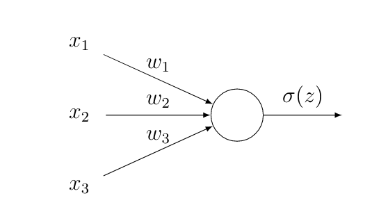
Figure fig_activate_neuron depicts the simplest possible ANN that consists of a single neuron. The neuron computes a weighted sum of the inputs and then applies an activation function [math]\actfun(z)[/math] to produce the output [math]\actfun(z)[/math]. The [math]\featureidx[/math]-th input of a neuron is assigned a parameter or weight [math]\weight_{\featureidx}[/math]. For a given choice of weights the ANN in Figure fig_activate_neuron represents a hypothesis map [math]h^{(\weights)}(\featurevec) = \actfun(z) = \actfun \big( \sum_{\featureidx} \weight_{\featureidx} \feature_{\featureidx} \big)[/math].

The ANN in Figure fig_activate_neuron defines a hypothesis space that is constituted by all maps [math]h^{(\weights)}[/math] obtained for different choices for the weights [math]\weights[/math] in Figure fig_activate_neuron. Note that the single-neuron ANN in Figure fig_activate_neuron reduces to a linear map when we use the activation function [math]\actfun(z) = z[/math]. However, even when we use a non-linear activation function in Figure fig_activate_neuron, the resulting hypothesis space is essentially the same as the space of linear maps \eqref{equ_lin_hypospace}. In particular, if we threshold the output of the ANN in Figure fig_activate_neuron to obtain a binary label, we will always obtain a linear classifier like logistic regression and SVM (see Section Logistic Regression and Section Support Vector Machines ).

Artificial neural network (ANN) consisting of a single neuron that implements a weighted summation [math]z=\sum_{\featureidx} \weight_{\featureidx} \feature_{\featureidx}[/math] of its inputs [math]\feature_{\featureidx}[/math] followed by applying a non-linear activation function [math]\actfun(z)[/math].

Deep learning methods use ANN consisting of many (thousands to millions) interconnected neurons .

In principle the interconnections between neurons can be arbitrary. One widely used approach however is to organize neurons as layers and place connections mainly between neurons in consecutive layers . Figure fig_ANN depicts an example for a ANN consisting of one hidden layer to represent a (parametrized) hypothesis [math]h^{(\weights)}: \mathbb{R}^{\featuredim} \rightarrow \mathbb{R}[/math].

ANN representation of a predictor [math]h^{(\weights)}(\featurevec)[/math] which maps the input (feature) vector [math]\featurevec=(\feature_{1},\feature_{2})^{T}[/math] to a predicted label (output) [math]h^{(\weights)}(\featurevec)[/math]. This ANN defines a hypothesis space consisting of all maps [math]h^{(\weights)}(\feature)[/math] obtained from all possible choices for the weights [math]\weights = (\weight_{1},\ldots,\weight_{9})^{T}[/math]

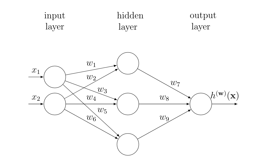
The first layer of the ANN in Figure fig_ANN is referred to as the input layer. The input layer reads in the feature vector [math]\featurevec \in \mathbb{R}^{\featuredim}[/math] of a data point. The features [math]\feature_{\featureidx}[/math] are then multiplied with the weights [math]\weight_{\featureidx,\featureidx'}[/math] associated with the link between the [math]\featureidx[/math]th input node (“neuron”) with the [math]\featureidx'[/math]th node in the middle (hidden) layer. The output of the [math]\featureidx'[/math]-th node in the hidden layer is given by [math]s_{\featureidx'}\!=\!\actfun( \sum_{\featureidx=1}^{\featuredim} \weight_{\featureidx,\featureidx'} \feature_{\featureidx} )[/math] with some (typically non-linear) activation function [math]\actfun: \mathbb{R} \rightarrow \mathbb{R}[/math]. The argument to the activation function is the weighted combination [math] \sum_{\featureidx=1}^{\featuredim} \weight_{\featureidx,\featureidx'} s_{\featureidx'}[/math] of the outputs [math]s_{\featureidx}[/math] of the nodes in the previous layer. For the ANN depicted in Figure fig_ANN, the output of neuron [math]s_{1}[/math] is [math]\actfun(z)[/math] with [math]z=\weight_{1,1}\feature_{1} + \weight_{1,2}\feature_{2}[/math].

The hypothesis map represented by an ANN is parametrized by the weights of the connections between neurons. Moreover, the resulting hypothesis map depends also on the choice for the activation functions of the individual neurons. These activation function are a design choice that can be adapted to the statistical properties of the data. However, a few particular choices for the activation function have proven useful in many important application domains. Two popular choices for the activation function used within ANNs are the sigmoid function [math]\actfun(z) = \frac{1}{1+\exp(-z)}[/math] or the rectified linear unit (ReLU) [math]\actfun(z) = \max\{0,z\}[/math]. ANNs using many, say [math]10[/math], hidden layers, is often referred to as a “deep net”. ML methods using hypothesis spaces obtained from deep ANN (deep net)s are known as deep learning methods .

It can be shown that an ANN with only one single (but arbitrarily large) hidden layer can approximate any given map [math]h: \featurespace \rightarrow \labelspace=\mathbb{R}[/math] to any desired accuracy . Deep learning methods often use a ANN with a relatively large number (more than hundreds) of hidden layers. We refer to a ANN with a relatively large number of hidden layers as a deep net.

There is empirical and theoretical evidence that using many hidden layers, instead of few but wide layers, is computationally and statistically favourable and . The hypothesis map [math]h^{(\weights)}[/math] represented by an ANN can be evaluated (to obtain the predicted label at the output) efficiently using message passing over the ANN. This message passing can be implemented using parallel and distributed computers. Moreover, the graphical representation of a parametrized hypothesis in the form of a ANN allows us to efficiently compute the gradient of the loss function via a (highly scalable) message passing procedure known as back-propagation . Being able to quickly compute gradients is instrumental for the efficiency of gradient based methods for learning a good choice for the ANN weights (see Chapter Gradient-Based Learning ).

Maximum Likelihood

For many applications it is useful to model the observed data points [math]\datapoint^{(\sampleidx)}[/math], with [math]\sampleidx=1,\ldots,\samplesize[/math], as iid realizations of a RV [math]\datapoint[/math] with probability distribution [math]\prob{\datapoint; \weights}[/math]. This probability distribution is parametrized by a parameter vector [math]\weights \in \mathbb{R}^{\featuredim}[/math]. A principled approach to estimating the parameter vector [math]\weights[/math] based on a set of iid realizations [math]\datapoint^{(1)},\ldots,\datapoint^{(\samplesize)}\sim \prob{\vz; \weights}[/math] is maximum likelihood estimation .

Maximum likelihood estimation can be interpreted as an ML problem with a hypothesis space parametrized by the parameter vector [math]\weights[/math]. Each element [math]h^{(\weights)}[/math] of the hypothesis space [math]\hypospace[/math] corresponds to one particular choice for the parameter vector [math]\weights[/math]. Maximum likelihood methods use the loss function

[[math]]\begin{equation} \label{equ_loss_ML} \loss{\datapoint}{h^{(\weights)}} \defeq - \log \prob{\datapoint; \weights}. \end{equation}[[/math]]

A widely used choice for the probability distribution [math]p \big( \datapoint; \weights \big)[/math] is a multivariate normal (Gaussian) distribution with mean [math]{\bm \mu}[/math] and covariance matrix [math]{\bf \Sigma}[/math], both of which constitute the parameter vector [math]\weights = ({\bm \mu}, {\bf \Sigma})[/math] (we have to reshape the matrix [math]{\bf \Sigma}[/math] suitably into a vector form). Given the iid realizations [math]\datapoint^{(1)},\ldots,\datapoint^{(\samplesize)} \sim p \big( \datapoint; \weights \big)[/math], the maximum likelihood estimates [math]\hat{\bm \mu}[/math], [math]\widehat{\bf \Sigma}[/math] of the mean vector and the covariance matrix are obtained via

[[math]]\begin{equation} \label{equ_max_likeli} \hat{\bm \mu}, \widehat{\bf \Sigma} = \argmin_{{\bm \mu} \in \mathbb{R}^{\featurelen},{\bf \Sigma} \in \mathbb{S}^{\featurelen}_{+}} (1/\samplesize) \sum_{\sampleidx=1}^{\samplesize} - \log p\big(\datapoint^{(\sampleidx)}; ({\bm \mu},{\bf \Sigma})\big). \end{equation}[[/math]]

The optimization in \eqref{equ_max_likeli} is over all possible choices for the mean vector [math]{\bm \mu} \in \mathbb{R}^{\featurelen}[/math] and the covariance matrix [math]{\bf \Sigma} \in \mathbb{S}^{\featurelen}_{+}[/math]. Here, [math]\mathbb{S}^{\featurelen}_{+}[/math] denotes the set of all positive semi-definite (psd) Hermitian [math]\featurelen \times \featurelen[/math] matrices.

The maximum likelihood problem \eqref{equ_max_likeli} can be interpreted as an instance of ERM using the particular loss function \eqref{equ_loss_ML}. The resulting estimates are given explicitly as

[[math]] \begin{equation} \label{equ_ML_mean_cov_Gauss} \hat{\bm \mu} = (1/\samplesize) \sum_{\sampleidx=1}^{\samplesize} \datapoint^{(\sampleidx)} \mbox{, and } \widehat{\bf \Sigma} = (1/\samplesize) \sum_{\sampleidx=1}^{\samplesize} (\datapoint^{(\sampleidx)} - \hat{\bm \mu})(\datapoint^{(\sampleidx)} - \hat{\bm \mu})^{T}. \end{equation} [[/math]]

Note that the expressions \eqref{equ_ML_mean_cov_Gauss} are only valid when the probability distribution of the data points is modelled as a multivariate normal distribution.

Nearest Neighbour Methods

Nearest neighbour (NN) methods are a family of ML methods that are characterized by a specific construction of the hypothesis space. NN methods can be applied to regression problems involving numeric labels (e.g., using label space [math]\labelspace=\mathbb{R}[/math] ) as well as for classification problems involving categorical labels (e.g., with label space [math]\labelspace = \{-1,1\}[/math]).

While nearest neighbour (NN) methods can be combined with arbitrary label spaces, they require the feature space to have a specific structure. NN methods require the feature space be a metric space that provides a measure for the distance between different feature vectors. We need a metric or distance measure to determine the nearest neighbour of a data point. A prominent example for a metric feature space is the Euclidean space [math]\mathbb{R}^{\featuredim}[/math]. The metric of [math]\mathbb{R}^{\featuredim}[/math] given by the Euclidean distance [math]\| \featurevec\!-\!\featurevec' \|[/math] between two vectors [math]\featurevec, \featurevec' \in \mathbb{R}^{\featuredim}[/math].

Consider a training set [math]\dataset = \{ (\featurevec^{(\sampleidx)},\truelabel^{(\sampleidx)}) \}_{\sampleidx=1}^{\samplesize}[/math] that consists of labeled data points. Thus, for each data point we know the features and the label value. Given such a training set, NN methods construct a hypothesis space that consist of piece-wise constant maps [math]h: \featurespace \rightarrow \labelspace[/math].

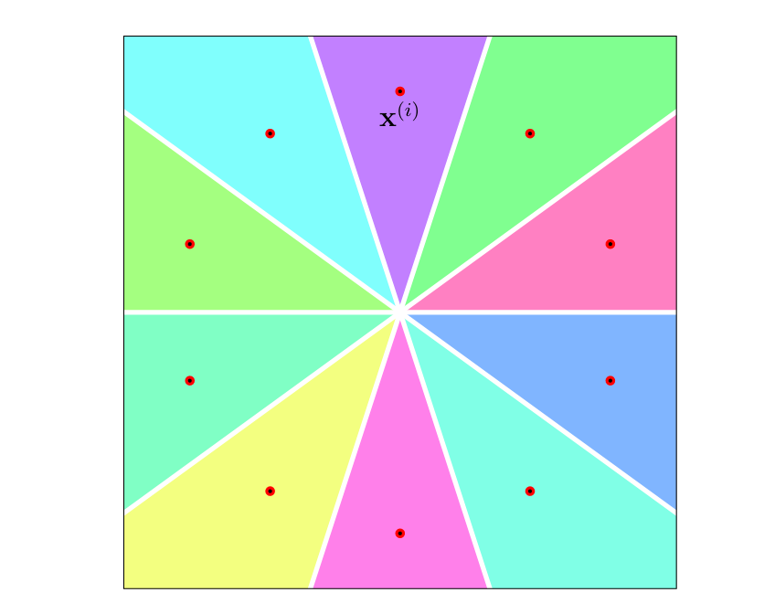
For any hypothesis [math]h[/math] in that space, the function value [math]h(\featurevec)[/math] obtained for a data point with features [math]\featurevec[/math] depends only on the (labels of the) [math]k[/math] nearest data points (smallest distance to [math]\featurevec[/math]) in the training set [math]\dataset[/math]. The number [math]k[/math] of NNs used to determine the function value [math]h(\featurevec)[/math] is a design (hyper-) parameter of a NN method. NN methods are also referred to as [math]k[/math]-NN methods to make their dependence on the parameter [math]k[/math] explicit.

Let us illustrate NN methods by considering a binary classification problem using an uneven number for [math]k[/math] (e.g., [math]k=3[/math] or [math]k=5[/math]).

The goal is to learn a hypothesis that predicts the binary label [math]\truelabel \in \{-1,1\}[/math] of a data point based on its feature vector [math]\featurevec \in \mathbb{R}^{\featuredim}[/math]. This learning task can make use of a training set [math]\dataset[/math] containing [math]\samplesize \gt k[/math] data points with known labels. Given a data point with features [math]\featurevec[/math], denote by [math]\neighbourhood{k}[/math] a set of [math]k[/math] data points in [math]\dataset[/math] whose feature vectors have smallest distance to [math]\featurevec[/math]. The number of data points in [math]\neighbourhood{k}[/math] whose label is [math]1[/math] is denoted [math]\samplesize^{(k)}_{1}[/math] and those with label value [math]-1[/math] is denoted [math]\samplesize^{(k)}_{-1}[/math]. The [math]k[/math]-NN method “learns” a hypothesis [math]\hat{h}[/math] given by

[[math]]\begin{equation} \label{equ_def_k_nn} \hat{h}(\featurevec) = \begin{cases} 1 & \mbox{ if } \samplesize^{(k)}_{1} \gt \samplesize^{(k)}_{-1} \\ - 1 & \mbox{ otherwise.} \end{cases} \end{equation}[[/math]]

It is important to note that, in contrast to the ML methods in Section Linear Regression - Section Deep Learning , the hypothesis space of [math]k[/math]-NN depends on a labeled dataset (training set) [math]\dataset[/math]. As a consequence, [math]k[/math]-NN methods need to access (and store) the training set whenever the compute a prediction (evaluate [math]h(\featurevec))[/math].

To compute the prediction [math]h(\featurevec)[/math] for a data point with features [math]\featurevec[/math], [math]k[/math]-NN needs to determine its NNs in the training set. When using a large training set this implies a large storage requirement for [math]k[/math]-NN methods. Moreover, [math]k[/math]-NN methods might be prone to revealing sensitive information with its predictions (see Exercise \ref{ex_privacy_k_nn}).

For a fixed [math]k[/math], NN methods do not require any parameter tuning. Such parameter tuning (or learning) is required linear regression, logistic regression and deep learning methods. In contrast, the hypothesis “learnt” by NN methods is characterized point-wise, for each possible value of features [math]\featurevec[/math], by the NN in the training set. Compared to the ML methods in Section Linear Regression - Section Deep Learning , NN methods do not require to solve (challenging) optimization problems for model parameters. Beside their low computational requirements (put aside the memory requirements), NN methods are also conceptually appealing as natural approximations of Bayes estimators (see and Exercise \ref{ex_k_nn_approximates_bayes}).

A hypothesis map [math]h[/math] for [math]k[/math]-NN with [math]k=1[/math] and feature space [math]\featurespace = \mathbb{R}^{2}[/math]

Deep Reinforcement Learning

Deep reinforcement learning (DRL) refers to a subset of ML problems and methods that revolve around the control of dynamic systems such as autonomous driving cars or cleaning robots . A DRL problem involves data points that represent the states of a dynamic system at different time instants [math]\timeidx=0,1,\ldots[/math]. The data points representing the state at some time instant [math]\timeidx[/math] is characterized by the feature vector [math]\featurevec^{(\timeidx)}[/math]. The entries of this feature vector are the individual features of the state at time [math]\timeidx[/math]. These features might be obtained via sensors, onboard-cameras or other ML methods (that predict the location of the dynamic system). The label [math]\truelabel^{(\timeidx)}[/math] of a data point might represent the optimal steering angle at time [math]\timeidx[/math].

DRL methods learn a hypothesis [math]h[/math] that delivers optimal predictions [math]\hat{\truelabel}^{(\timeidx)} \defeq h \big( \featurevec^{(\timeidx)} \big)[/math] for the optimal steering angle [math]\truelabel^{(\timeidx)}[/math]. As their name indicates, DRL methods use hypothesis spaces obtained from a deep net (see Section Deep Learning ). The quality of the prediction [math]\hat{\truelabel}^{(\timeidx)}[/math] obtained from a hypothesis is measured by the loss [math]\loss{\big(\featurevec^{(\timeidx)},\truelabel^{(\timeidx)} \big)}{h} \defeq - \reward^{(\timeidx)}[/math] with a reward signal [math]\reward^{(\timeidx)}[/math]. This reward signal might be obtained from a distance (collision avoidance) sensor or low-level characteristics of an on-board camera snapshot.

The (negative) reward signal [math]- \reward^{(\timeidx)}[/math] typically depends on the feature vector [math]\featurevec^{(\timeidx)}[/math] and the discrepancy between optimal steering direction [math]\truelabel^{(\timeidx)}[/math] (which is unknown) and its prediction [math]\hat{\truelabel}^{(\timeidx)} \defeq h \big( \featurevec^{(\timeidx)} \big)[/math]. However, what sets DRL methods apart from other ML methods such as linear regression (see Section Linear Regression ) or logistic regression (see Section Logistic Regression ) is that they can evaluate the loss function only point-wise [math]\loss{\big(\featurevec^{(\timeidx)},\truelabel^{(\timeidx)} \big)}{h}[/math] for the specific hypothesis [math]h[/math] that has been used to compute the prediction [math]\hat{\truelabel}^{(\timeidx)} \defeq h \big( \featurevec^{(\timeidx)} \big)[/math] at time instant [math]\timeidx[/math]. This is fundamentally different from linear regression that uses the squared error loss which can be evaluated for every possible hypothesis [math]h \in \hypospace[/math].

LinUCB

ML methods are instrumental for various recommender systems . A basic form of a recommender system amount to chose at some time instant [math]\timeidx[/math] the most suitable item (product, song, movie) among a finite set of alternatives [math]\actionidx = 1,\ldots,\nractions[/math]. Each alternative is characterized by a feature vector [math]\featurevec^{(\timeidx,\actionidx)}[/math] that varies between different time instants.

The data points arising in recommender systems might represent time instants [math]\timeidx[/math] at which recommendations are computed. The data point at time [math]\timeidx[/math] is characterized by a feature vector

[[math]]\begin{equation} \label{equ_stacked_feature_LinUCB} \featurevec^{(\timeidx)} = \big( \big(\featurevec^{(\timeidx,1)}\big)^{T},\ldots,\big( \featurevec^{(\timeidx,\nractions)} \big)^{T} \big)^{T}. \end{equation}[[/math]]

The feature vector [math]\featurevec^{(\timeidx)}[/math] is obtained by stacking the feature vectors of alternatives at time [math]\timeidx[/math] into a single long feature vector. The label of the data point [math]\timeidx[/math] is a vector of rewards [math]\labelvec^{(\timeidx)} \defeq \big ( \reward_{1}^{(\timeidx)}, \ldots,\reward_{\nractions}^{(\timeidx)}\big)^{T} \in \mathbb{R}^{\nractions}[/math]. The entry [math]\reward_{\actionidx}^{(\timeidx)}[/math] represents the reward obtained by choosing (recommending) alternative [math]\actionidx[/math] (with features [math]\featurevec^{(\timeidx,\actionidx)}[/math]) at time [math]\timeidx[/math]. We might interpret the reward [math]\reward^{(\timeidx,\actionidx)}[/math] as an indicator if the costumer actually buys the product corresponding to the recommended alternative [math]\actionidx[/math].

The ML method LinUCB (the name seems to be inspired by the terms “linear” and “upper confidence bound” (UCB)) aims at learning a hypothesis [math]h[/math] that allows to predict the rewards [math]\labelvec^{(\sampleidx)}[/math] based on the feature vector [math]\featurevec^{(\timeidx)}[/math] \eqref{equ_stacked_feature_LinUCB}. As its hypothesis space [math]\hypospace[/math], LinUCB uses the space of linear maps from the stacked feature vectors [math]\mathbb{R}^{\featurelen \nractions}[/math] to the space of reward vectors [math]\mathbb{R}^{\nractions}[/math]. This hypothesis space can be parametrized by matrices [math]\mW \in \mathbb{R}^{\nractions \times \featurelen \nractions}[/math]. Thus, LinUCB learns a hypothesis that computes predicted rewards via

[[math]]\begin{equation} \widehat{\labelvec}^{(\timeidx)} \defeq \mW \featurevec^{(\timeidx)}. \end{equation}[[/math]]

The entries of [math]\widehat{\labelvec}^{(\timeidx)} = \big( \hat{\reward}_{1}^{(\timeidx)},\ldots,\hat{\reward}_{\nractions}^{(\timeidx)}\big)[/math] are predictions of the individual rewards [math]\reward^{(\timeidx,\actionidx)}[/math]. It seems natural to recommend at time [math]\timeidx[/math] the alternative [math]\actionidx[/math] whose predicted reward is maximum. However, it turns out that this approach is sub-optimal as it prevents the recommender system from learning the optimal predictor map [math]\mW[/math].

Loosely speaking, LinUCB tries out (explores) each alternative [math]\actionidx \in \{1,\ldots,\nractions\}[/math] sufficiently often to obtain a sufficient amount of training data for learning a good weight matrix [math]\mW[/math]. At time [math]\timeidx[/math], LinUCB chooses the alternative [math]\actionidx^{(\timeidx)}[/math] that maximizes the quantity

[[math]]\begin{equation} \label{equ_linucb_bound} \hat{\reward}_{\actionidx}^{(\timeidx)} + R(\timeidx,\actionidx) \mbox{ , } \actionidx = 1,\ldots,\nractions. \end{equation}[[/math]]

We can think of the component [math]R(\timeidx,\actionidx)[/math] as a form of confidence interval. It is constructed such that \eqref{equ_linucb_bound} upper bounds the actual reward [math]\reward_{\actionidx}^{(\timeidx)}[/math] with a prescribed level of confidence (or probability). The confidence term [math]R(\timeidx,\actionidx)[/math] depends on the feature vectors [math]\featurevec^{(\timeidx',\actionidx)}[/math] of the alternative [math]\actionidx[/math] at previous time instants [math]\timeidx' \lt \timeidx[/math]. Thus, at each time instant [math]\timeidx[/math], LinUCB chooses the alternative [math]\actionidx[/math] that results in the largest upper confidence bound (UCB) \eqref{equ_linucb_bound} on the reward (hence the “UCB” in LinUCB). We refer to the relevant literature on sequential learning (and decision making) for more details on the LinUCB .

Notes

References