guide:De57bb5bf8: Difference between revisions
m (1 revision imported) |
mNo edit summary |
||
| Line 171: | Line 171: | ||
{{cite arXiv|last=Herberg|first=Evelyn|year=2023|title=Lecture Notes: Neural Network Architectures|eprint=2304.05133|class=cs.LG}} | {{cite arXiv|last=Herberg|first=Evelyn|year=2023|title=Lecture Notes: Neural Network Architectures|eprint=2304.05133|class=cs.LG}} | ||
==References== | ==References== | ||
Revision as of 23:04, 27 June 2023
The Neural Networks we introduced so far rely on the assumption of independence among the training and test examples. They process one data point at a time, which is no problem for data sets, in which every data point is generated independently. However, for sequential data that occurs in machine translation, speech recognition, sentiment classification, etc., the dependence is highly relevant to the task.
Recurrent Neural Networks (RNNs), cf. e.g. [1](Section 10) and [2](Section 8.1), are connectionist models that capture the dynamics of sequences via cycles in the network of nodes. Unlike standard FNNs, recurrent neural networks retain a state that can represent information from an arbitrarily long context window.
Example
Translate a given english input sentence [math]u[/math], consisting of [math]T_{\operatorname{in}}[/math] words [math]u^{\lt t \gt}, t=1,\ldots,T_{\operatorname{in}}[/math], e.g.
to a german output sentence [math]y[/math], consisting of [math]T_{\operatorname{out}}[/math] words [math]y^{\lt t \gt}, t=1,\ldots,T_{\operatorname{out}}[/math]. Hopefully, the output will be something like
A comparison of FNN and RNN architecture can be seen in Figure. For simplicity of notation we condense all hidden layers of the FNN into a representative computation node [math]h[/math].
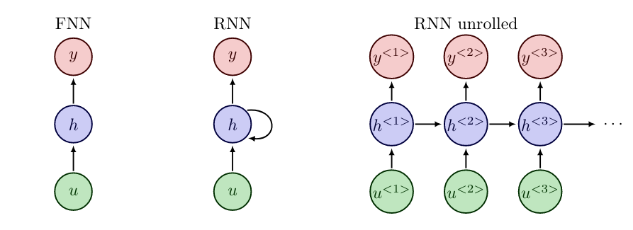
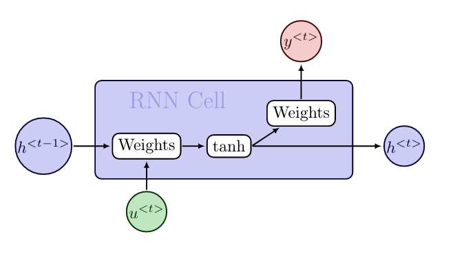
In RNNs the computation nodes [math]h[/math] are often called RNN cells, cf. [1](Section 10.2). A RNN cell for a time instance [math]t[/math] takes as an input [math]u^{\lt t \gt}[/math] and [math]h^{\lt t-1\gt}[/math], and computes the outputs [math]h^{\lt t \gt}[/math] and [math]y^{\lt t \gt}[/math], cf. Figure. More specifically for all [math]t=1,\ldots,T_{\operatorname{out}}[/math]
The equations \eqref{eq:RNN1} and \eqref{eq:RNN2} describe the forward propagation in RNNs. Here, [math][h^{\lt t-1\gt} ; u^{\lt t \gt}][/math] denotes the concatenation of the vectors, and [math]h^{\lt0\gt}[/math] is set to a vector of zeros, so that we do not need to formulate a special case for [math]t=1[/math]. Depending on the application, a softmax function may be applied to [math]W_{\operatorname{out}} h^{\lt t \gt}[/math] to get the output [math]y^{\lt t \gt}[/math].
It may happen that input and output have different lengths [math]T_{\operatorname{in}} \neq T_{\operatorname{out}}[/math], see e.g. Example. Depending on the task and the structure of the data, there exist various types of RNN architectures, cf. [2](Section 8.1) and Figure:
- one to many, e.g. image description (image to sentence),
- many to one, e.g. sentiment analysis (video to word),
- many to many, e.g. machine translation (sentence to sentence), like Example,
- many to many, e.g. object tracking (video to object location per frame).
We note that the weights [math]W_{\operatorname{in}}, W_{\operatorname{out}}[/math] and bias [math]b[/math] in \eqref{eq:RNN1} and \eqref{eq:RNN2} do not change over time, but coincide for all temporal layers of the RNN. Sharing the variables allows the RNN to model variable length sequences, whereas if we had specific parameters for each value of the order parameter, we could not generalize to sequence lengths not seen during training. Typically, [math]\sigma = \tanh[/math] is chosen in RNNs, and this does also not vary between the layers. To obtain a complete optimization problem, we still need a loss function [math]\mathscr{L}[/math], since the RNN represents only the network [math]\mathcal{F}[/math]. To this end, each output [math]y^{\lt t \gt}[/math] is evaluated with a loss function [math]\mathscr{L}^{\lt t \gt}[/math] and the final loss is computed by taking the sum over all time instances
Here, as usual, [math]\theta[/math] contains the weights [math]W_{\operatorname{in}},W_{\operatorname{out}}[/math], and bias [math]b[/math].
Variants of RNNs
We briefly introduce two popular variants of RNNs.
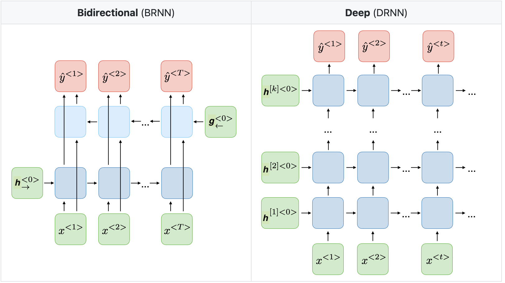
In many applications the output at time [math]t[/math] should be a prediction depending on the whole input sequence, not only the "earlier" inputs [math]u^{\lt i \gt}[/math] with [math]i \leq t[/math]. E.g., in speech recognition, the correct interpretation of the current sound as a phoneme may depend on the next few phonemes because of co-articulation and potentially may even depend on the next few words because of the linguistic dependencies between nearby words. As a remedy, we can combine a forward-going RNN and a backward-going RNN, which is then called a Bidirectional RNN, [1](Section 10.3). This architecture allows to compute an output [math]y^{\lt t \gt}[/math] that depends on both the past and the future inputs, but is most sensitive to the input values around time [math]t[/math]. Figure (left) illustrates the typical bidirectional RNN, with [math]h^{\lt t \gt}[/math] and [math]g^{\lt t \gt}[/math] representing the states of the sub-RNNs that move forward and backward through time, respectively.
Another variant of RNNs is the Deep RNN, [1](Section 10.5). As seen in FNNs, Section Feedforward Neural Network , multiple hidden layers allow the network to have a higher expressiveness. Similarly, a RNN can be made deep by stacking RNN cells, see Figure (right).
Long term dependencies
In this section we investigate one of the main challenges, that a RNN can encounter, cf. [1](Section 10.7). Consider the following illustrative example.
Example
Predict the next word in the sequence:
- The cat, which ..., was ...
- The cats, which ..., were ...
Here, depending on whether we are talking about one cat or multiple cats the verb has to be adjusted. The "..." part in the sentence can be very extensive, so that the dependence becomes long.
The gradient from the output [math]y^{\lt t \gt}[/math] with large [math]t[/math] has to propagate back through many layers to affect weights in early layers. Here, the vanishing gradient and exploding gradient problems (cf. Section ResNet ) may occur and hinder training. The exploding gradient problem can be solved relatively robust by gradient clipping, see e.g. [1](Section 10.11.1). The idea is quite simple. If a gradient [math]\partial_{\theta_i}{\mathscr{L}}[/math], with respect to some variable [math]\theta_i[/math] gets too large, we rescale it. I.e. if [math]\| \partial_{\theta_i}{\mathscr{L}}\| \geq C \in \mathbb{R}[/math] for a hyperparameter [math]C[/math], we set
Let us remark that this is a heuristic approach. In contrast, the vanishing gradient problem is more difficult to solve.
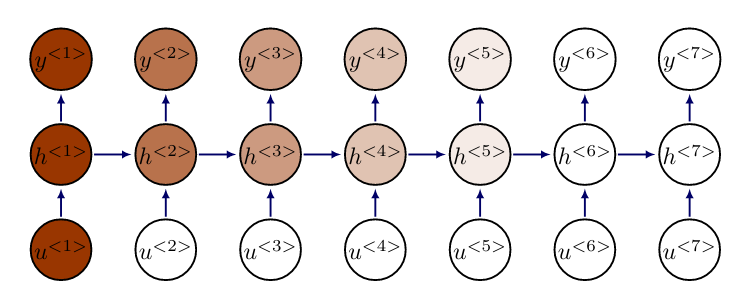
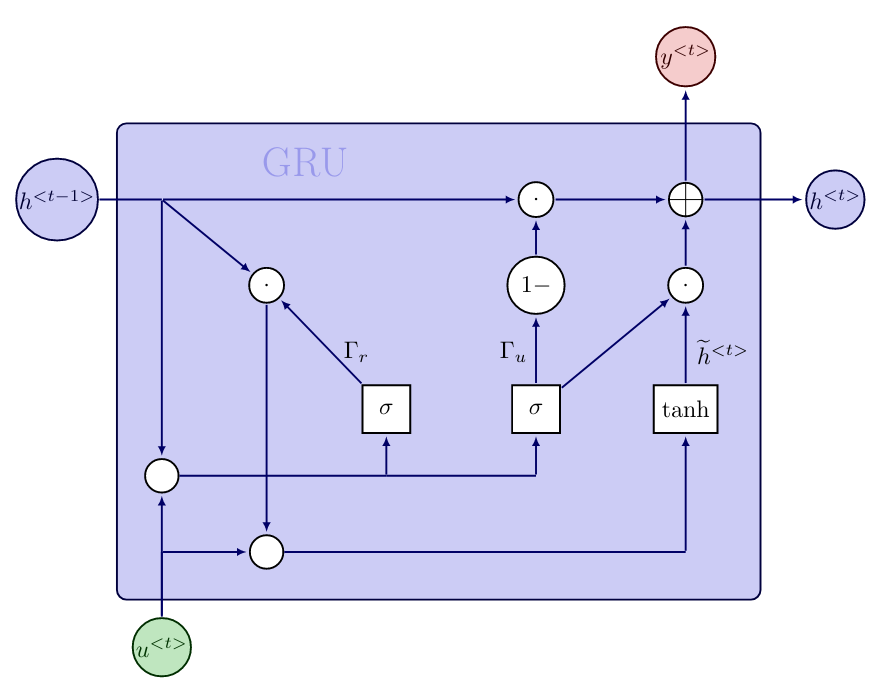
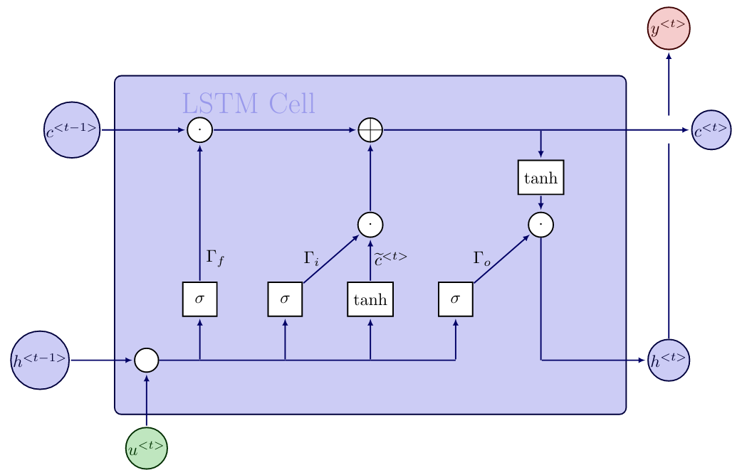
A common remedy is to modify the RNN cell so that it can capture long term dependencies better, and avoids vanishing gradients. Two popular options are Gated Recurrent Unit (GRU) from 2014 [3], and the cell architecture as suggested already in 1997 in Long Short Term Memory (LSTM) networks [4]. The core idea in both cell architectures is to add gating mechanisms. These gates have a significant influence on whether, and how severely, the input and previous hidden state influence the output and new hidden state. Additionally, the gating mechanism helps to solve the vanishing gradient problem.
Gated Recurrent Unit
The gated recurrent unit has a reset (or relevance) gate [math]\Gamma_r[/math] and an update gate [math]\Gamma_u[/math]. The computations for one unit are as follows
The computations of the hidden state candidate [math]\widetilde{h}^{\lt t \gt}[/math] and the output [math]y^{\lt t \gt}[/math] resemble the computations in the RNN cell \eqref{eq:RNN1} and \eqref{eq:RNN2}, respectively. However, e.g. if [math]\Gamma_u = 0[/math], then the new hidden state will coincide with the previous hidden state and the candidate will not be taken into account. Also, the GRU has significantly more variables per cell, in comparison with the standard RNN cell.
Long Short Term Memory
The key to LSTM networks is that in addition to the hidden state, there also exists a cell state [math]c^{\lt t \gt}[/math], which is propagated through the network. It can be understood like a conveyor belt, which only has minor interactions and runs down the entire chain of LSTM cells, see Figure. This allows information to flow through the network easily. In contrast to GRU, the LSTM cell contains three gates: the forget gate [math]\Gamma_f[/math], input gate [math]\Gamma_i[/math] and output gate [math]\Gamma_o[/math].
Language processing
An important application of RNNs is language processing, e.g. machine translation, see Example. In such tasks the words need to be represented, so that the RNN can work with them. Furthermore, we need a way to deal with punctuation marks, and an indicator for the end of a sentence.
To represent the words, we form a dictionary. For the english language we will end up with a vector containing more than 10000 words. Intuitively, we sort the words alphabetically and to simplify computations we use a one-hot representation. E.g., if "the" is the 8367th word in the english dictionary vector, we represent the first input
with the 8367th unit vector. This allows for an easy way to measure correctness in supervised learning and later on we can use the dictionary to recover the words. Additionally, it is common to create a token for unknown words, which are not in the dictionary. Punctuation marks can either be ignored, or we also create tokens for them. However, the dictionary should at least contain an "end of sentence" token to separate sentences from each other.
General references
Herberg, Evelyn (2023). "Lecture Notes: Neural Network Architectures". arXiv:2304.05133 [cs.LG].
References
- 1.0 1.1 1.2 1.3 1.4 1.5 I. Goodfellow, Y. Bengio, and A. Courville. (2016). Deep learning. MIT Press.CS1 maint: multiple names: authors list (link)
- 2.0 2.1 Geiger, A. (2021), Deep Learning Lecture Notes
- Cho, K. and Van Merriénboer, B. and Gulcehre, C. and Bahdanau, D. and Bougares, F. and Schwenk, H. and Bengio, Y. (2014). "Learning phrase representations using RNN encoder-decoder for statistical machine translation". arXiv preprint arXiv:1406.1078.
- Hochreiter, S. and Schmidhuber, J.f (1997). "Long short-term memory". Neural computation 9. MIT press.
- He, K. and Zhang, X. and Ren, S. and Sun, J. (2016). "Deep residual learning for image recognition". Proceedings of the IEEE conference on computer vision and pattern recognition.CS1 maint: uses authors parameter (link)
