guide:509f7f160f

[math] \( % Generic syms \newcommand\defeq{:=} \newcommand{\Tt}[0]{\boldsymbol{\theta}} \newcommand{\XX}[0]{{\cal X}} \newcommand{\ZZ}[0]{{\cal Z}} \newcommand{\vx}[0]{{\bf x}} \newcommand{\vv}[0]{{\bf v}} \newcommand{\vu}[0]{{\bf u}} \newcommand{\vs}[0]{{\bf s}} \newcommand{\vm}[0]{{\bf m}} \newcommand{\vq}[0]{{\bf q}} \newcommand{\mX}[0]{{\bf X}} \newcommand{\mC}[0]{{\bf C}} \newcommand{\mA}[0]{{\bf A}} \newcommand{\mL}[0]{{\bf L}} \newcommand{\fscore}[0]{F_{1}} \newcommand{\sparsity}{s} \newcommand{\mW}[0]{{\bf W}} \newcommand{\mD}[0]{{\bf D}} \newcommand{\mZ}[0]{{\bf Z}} \newcommand{\vw}[0]{{\bf w}} \newcommand{\D}[0]{{\mathcal{D}}} \newcommand{\mP}{\mathbf{P}} \newcommand{\mQ}{\mathbf{Q}} \newcommand{\E}[0]{{\mathbb{E}}} \newcommand{\vy}[0]{{\bf y}} \newcommand{\va}[0]{{\bf a}} \newcommand{\vn}[0]{{\bf n}} \newcommand{\vb}[0]{{\bf b}} \newcommand{\vr}[0]{{\bf r}} \newcommand{\vz}[0]{{\bf z}} \newcommand{\N}[0]{{\mathcal{N}}} \newcommand{\vc}[0]{{\bf c}} % Statistics and Probability Theory \newcommand{\errprob}{p_{\rm err}} \newcommand{\prob}[1]{p({#1})} \newcommand{\pdf}[1]{p({#1})} \def \expect {\mathbb{E} } % Machine Learning Symbols \newcommand{\biasterm}{B} \newcommand{\varianceterm}{V} \newcommand{\neighbourhood}[1]{\mathcal{N}^{(#1)}} \newcommand{\nrfolds}{k} \newcommand{\mseesterr}{E_{\rm est}} \newcommand{\bootstrapidx}{b} %\newcommand{\modeldim}{r} \newcommand{\modelidx}{l} \newcommand{\nrbootstraps}{B} \newcommand{\sampleweight}[1]{q^{(#1)}} \newcommand{\nrcategories}{K} \newcommand{\splitratio}[0]{{\rho}} \newcommand{\norm}[1]{\Vert {#1} \Vert} \newcommand{\sqeuclnorm}[1]{\big\Vert {#1} \big\Vert^{2}_{2}} \newcommand{\bmx}[0]{\begin{bmatrix}} \newcommand{\emx}[0]{\end{bmatrix}} \newcommand{\T}[0]{\text{T}} \DeclareMathOperator*{\rank}{rank} %\newcommand\defeq{:=} \newcommand\eigvecS{\hat{\mathbf{u}}} \newcommand\eigvecCov{\mathbf{u}} \newcommand\eigvecCoventry{u} \newcommand{\featuredim}{n} \newcommand{\featurelenraw}{\featuredim'} \newcommand{\featurelen}{\featuredim} \newcommand{\samplingset}{\mathcal{M}} \newcommand{\samplesize}{m} \newcommand{\sampleidx}{i} \newcommand{\nractions}{A} \newcommand{\datapoint}{\vz} \newcommand{\actionidx}{a} \newcommand{\clusteridx}{c} \newcommand{\sizehypospace}{D} \newcommand{\nrcluster}{k} \newcommand{\nrseeds}{s} \newcommand{\featureidx}{j} \newcommand{\clustermean}{{\bm \mu}} \newcommand{\clustercov}{{\bm \Sigma}} \newcommand{\target}{y} \newcommand{\error}{E} \newcommand{\augidx}{b} \newcommand{\task}{\mathcal{T}} \newcommand{\nrtasks}{T} \newcommand{\taskidx}{t} \newcommand\truelabel{y} \newcommand{\polydegree}{r} \newcommand\labelvec{\vy} \newcommand\featurevec{\vx} \newcommand\feature{x} \newcommand\predictedlabel{\hat{y}} \newcommand\dataset{\mathcal{D}} \newcommand\trainset{\dataset^{(\rm train)}} \newcommand\valset{\dataset^{(\rm val)}} \newcommand\realcoorspace[1]{\mathbb{R}^{\text{#1}}} \newcommand\effdim[1]{d_{\rm eff} \left( #1 \right)} \newcommand{\inspace}{\mathcal{X}} \newcommand{\sigmoid}{\sigma} \newcommand{\outspace}{\mathcal{Y}} \newcommand{\hypospace}{\mathcal{H}} \newcommand{\emperror}{\widehat{L}} \newcommand\risk[1]{\expect \big \{ \loss{(\featurevec,\truelabel)}{#1} \big\}} \newcommand{\featurespace}{\mathcal{X}} \newcommand{\labelspace}{\mathcal{Y}} \newcommand{\rawfeaturevec}{\mathbf{z}} \newcommand{\rawfeature}{z} \newcommand{\condent}{H} \newcommand{\explanation}{e} \newcommand{\explainset}{\mathcal{E}} \newcommand{\user}{u} \newcommand{\actfun}{\sigma} \newcommand{\noisygrad}{g} \newcommand{\reconstrmap}{r} \newcommand{\predictor}{h} \newcommand{\eigval}[1]{\lambda_{#1}} \newcommand{\regparam}{\lambda} \newcommand{\lrate}{\alpha} \newcommand{\edges}{\mathcal{E}} \newcommand{\generror}{E} \DeclareMathOperator{\supp}{supp} %\newcommand{\loss}[3]{L({#1},{#2},{#3})} \newcommand{\loss}[2]{L\big({#1},{#2}\big)} \newcommand{\clusterspread}[2]{L^{2}_{\clusteridx}\big({#1},{#2}\big)} \newcommand{\determinant}[1]{{\rm det}({#1})} \DeclareMathOperator*{\argmax}{argmax} \DeclareMathOperator*{\argmin}{argmin} \newcommand{\itercntr}{r} \newcommand{\state}{s} \newcommand{\statespace}{\mathcal{S}} \newcommand{\timeidx}{t} \newcommand{\optpolicy}{\pi_{*}} \newcommand{\appoptpolicy}{\hat{\pi}} \newcommand{\dummyidx}{j} \newcommand{\gridsizex}{K} \newcommand{\gridsizey}{L} \newcommand{\localdataset}{\mathcal{X}} \newcommand{\reward}{r} \newcommand{\cumreward}{G} \newcommand{\return}{\cumreward} \newcommand{\action}{a} \newcommand\actionset{\mathcal{A}} \newcommand{\obstacles}{\mathcal{B}} \newcommand{\valuefunc}[1]{v_{#1}} \newcommand{\gridcell}[2]{\langle #1, #2 \rangle} \newcommand{\pair}[2]{\langle #1, #2 \rangle} \newcommand{\mdp}[5]{\langle #1, #2, #3, #4, #5 \rangle} \newcommand{\actionvalue}[1]{q_{#1}} \newcommand{\transition}{\mathcal{T}} \newcommand{\policy}{\pi} \newcommand{\charger}{c} \newcommand{\itervar}{k} \newcommand{\discount}{\gamma} \newcommand{\rumba}{Rumba} \newcommand{\actionnorth}{\rm N} \newcommand{\actionsouth}{\rm S} \newcommand{\actioneast}{\rm E} \newcommand{\actionwest}{\rm W} \newcommand{\chargingstations}{\mathcal{C}} \newcommand{\basisfunc}{\phi} \newcommand{\augparam}{B} \newcommand{\valerror}{E_{v}} \newcommand{\trainerror}{E_{t}} \newcommand{\foldidx}{b} \newcommand{\testset}{\dataset^{(\rm test)} } \newcommand{\testerror}{E^{(\rm test)}} \newcommand{\nrmodels}{M} \newcommand{\benchmarkerror}{E^{(\rm ref)}} \newcommand{\lossfun}{L} \newcommand{\datacluster}[1]{\mathcal{C}^{(#1)}} \newcommand{\cluster}{\mathcal{C}} \newcommand{\bayeshypothesis}{h^{*}} \newcommand{\featuremtx}{\mX} \newcommand{\weight}{w} \newcommand{\weights}{\vw} \newcommand{\regularizer}{\mathcal{R}} \newcommand{\decreg}[1]{\mathcal{R}_{#1}} \newcommand{\naturalnumbers}{\mathbb{N}} \newcommand{\featuremapvec}{{\bf \Phi}} \newcommand{\featuremap}{\phi} \newcommand{\batchsize}{B} \newcommand{\batch}{\mathcal{B}} \newcommand{\foldsize}{B} \newcommand{\nriter}{R} [/math]

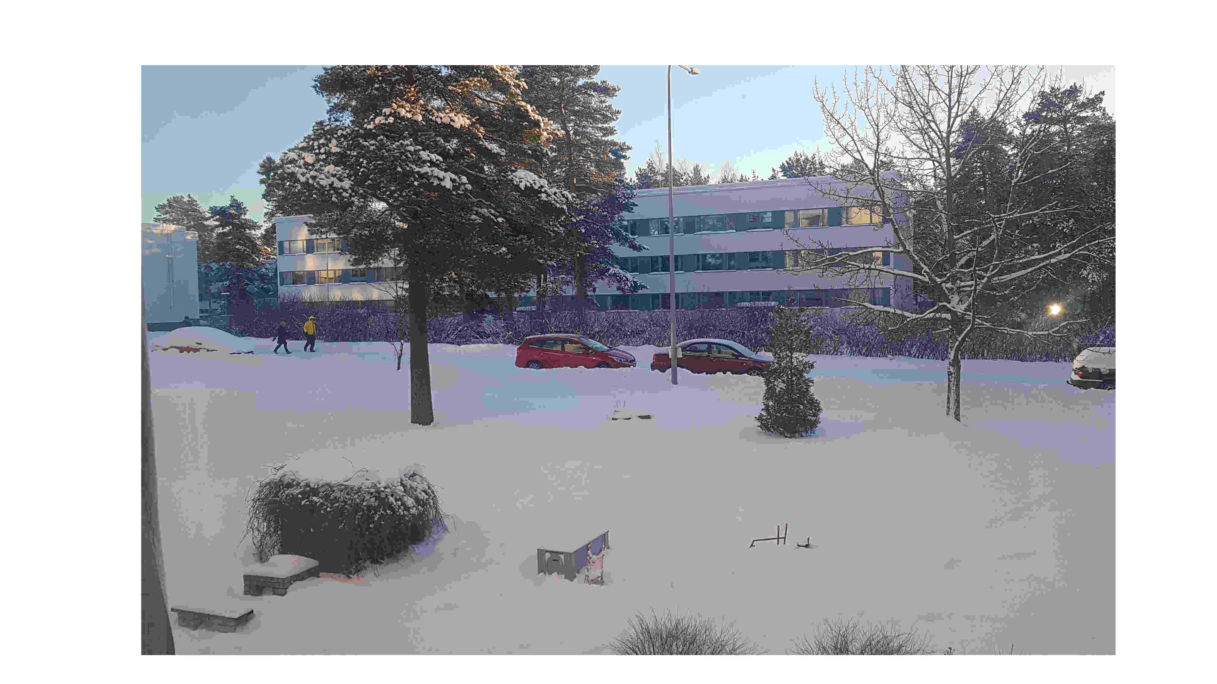
Consider waking up one winter morning in Finland and looking outside the window (see Figure fig:skiday ). It seems to become a nice sunny day which is ideal for a ski trip. To choose the right gear (clothing, wax) it is vital to have some idea for the maximum daytime temperature which is typically reached around early afternoon. If we expect a maximum daytime temperature of around plus [math]5[/math] degrees, we might not put on the extra warm jacket but rather take only some extra shirt for change.

Looking outside the window during the morning of a winter day in Finland.

We can use ML to learn a predictor for the maximum daytime temperature for the specific day depicted in Figure fig:skiday . The prediction shall be based solely on the minimum temperature observed in the morning of that day. ML methods can learn a predictor in a data-driven fashion using historic weather observations provided by the Finnish Meteorological Institute (FMI). We can download the recordings of minimum and maximum daytime temperature for the most recent days and denote the resulting dataset by

[[math]] \begin{equation}\label{equ_FMI_data} \dataset = \big\{ \datapoint^{(1)},\ldots,\datapoint^{(\samplesize)} \big\}. \end{equation}[[/math]]

Each data point [math]\datapoint^{(\sampleidx)} = \big(\feature^{(\sampleidx)},\truelabel^{(\sampleidx)}\big)[/math], for [math]\sampleidx=1,\ldots,\samplesize[/math], represents some previous day for which the minimum and maximum daytime temperature [math]\feature^{(\sampleidx)}[/math] and [math]\truelabel^{(\sampleidx)}[/math] has been recorded. We depict the data \eqref{equ_FMI_data} in fig_scatterplot_temp_FMI. Each dot in fig_scatterplot_temp_FMI represents a specific day with minimum temperature [math]\feature[/math] and maximum temperature [math]\truelabel[/math].

Each dot represents a specific day that is characterized by its minimum daytime temperature [math]\feature[/math] as feature and its maximum daytime temperature [math]\truelabel[/math] as label. These temperatures are measured at some FMI weather station.

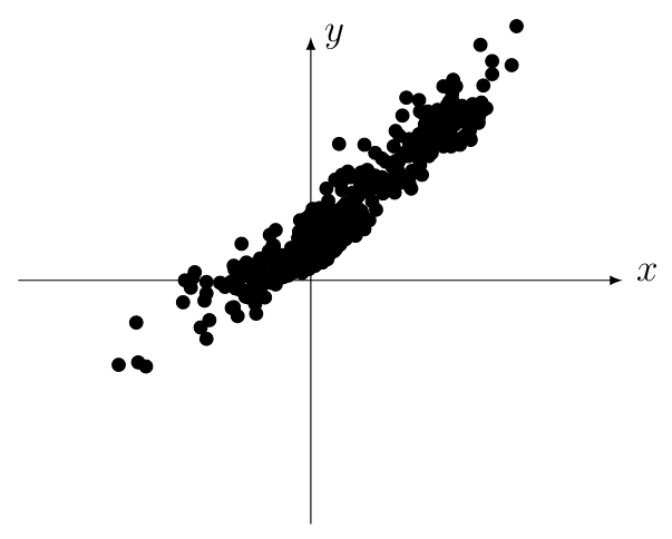
ML methods learn a hypothesis [math]h(\feature)[/math], that reads in the minimum temperature [math]\feature[/math] and delivers a prediction (forecast or approximation) [math]\hat{\truelabel} = h(\feature)[/math] for the maximum daytime temperature [math]\truelabel[/math]. Every practical ML method uses a particular hypothesis space out of which the hypothesis [math]h[/math] is chosen. This hypothesis space of candidates for the hypothesis map is an important design choice and might be based on domain knowledge.

In what follows, we illustrate how to use domain knowledge to motivate a choice for the hypothesis space. Let us assume that the minimum and maximum daytime temperature of an arbitrary day are approximately related via

[[math]] \begin{equation}\label{equ_initial_hypo_FMI} \truelabel \approx \weight_{1} \feature + \weight_{0} \mbox{ with some weights } \weight_{1} \in \mathbb{R}_{+}, \weight_{0} \in \mathbb{R}. \end{equation}[[/math]]

The assumption \eqref{equ_initial_hypo_FMI} reflects the intuition (domain knowledge) that the maximum daytime temperature [math]\truelabel[/math] should be higher for days with a higher minimum daytime temperature [math]\feature[/math]. The assumption \eqref{equ_initial_hypo_FMI} contains two weights [math]\weight_{1}[/math] and [math]\weight_{0}[/math]. These weights are tuning parameters that allow for some flexibility in our assumption. We require the weight [math]\weight_{1}[/math] to be non-negative but otherwise leave these weights unspecified for the time being. The main subject of this book are ML methods that can be used to learn suitable values for the weights [math]\weight_{1}[/math] and [math]\weight_{0}[/math] in a data-driven fashion.

Before we detail how ML can be used to find or learn good values for the weights [math]\weight_{0}[/math] in [math]\weight_{1}[/math] in \eqref{equ_initial_hypo_FMI} let us interpret them. The weight [math]\weight_{1}[/math] in \eqref{equ_initial_hypo_FMI} can be interpreted as the relative increase in the maximum daytime temperature for an increased minimum daytime temperature. Consider an earlier day with recorded maximum daytime temperature of [math]10[/math] degrees and minimum daytime temperature of [math]0[/math] degrees. The assumption \eqref{equ_initial_hypo_FMI} then means that the maximum daytime temperature for another day with minimum temperature of [math]+1[/math] degrees would be [math]10 + \weight_{1}[/math] degrees. The second weight [math]\weight_{0}[/math] in our assumption \eqref{equ_initial_hypo_FMI} can be interpreted as the maximum daytime temperature that we anticipate for a day with minimum daytime temperature equal to [math]0[/math].

Given the assumption \eqref{equ_initial_hypo_FMI}, it seems reasonable to restrict the ML method to only consider linear maps

[[math]] \begin{equation}\label{equ_def_linear_map_scalar} h(\feature) \defeq \weight_{1} \feature + \weight_{0} \mbox{ with some weights } w_{1} \in \mathbb{R}_{+},w_{0} \in \mathbb{R}. \end{equation}[[/math]]

Since we require [math]\weight_{1}\!\geq\!0[/math], the map \eqref{equ_def_linear_map_scalar} is monotonically increasing with respect to the argument [math]\feature[/math]. Therefore, the prediction [math]h(\feature)[/math] for the maximum daytime temperature becomes higher with higher minimum daytime temperature [math]\feature[/math].

The expression \eqref{equ_def_linear_map_scalar} defines a whole ensemble of hypothesis maps. Each individual map corresponding to a particular choice for [math]\weight_{1} \geq 0[/math] and [math]\weight_{0}[/math]. We refer to such an ensemble of potential predictor maps as the model or hypothesis space that is used by a ML method.

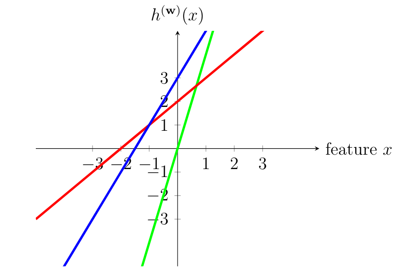
We say that the map \eqref{equ_def_linear_map_scalar} is parametrized by the vector [math]\weights= \big(\weight_{1},\weight_{0}\big)^{T}[/math] and indicate this by writing [math]h^{(\weights)}[/math]. For a given parameter vector [math]\weights= \big(\weight_{1},\weight_{0}\big)^{T}[/math], we obtain the map [math]h^{(\weights)}(\feature) = \weight_{1} \feature +\weight_{0}[/math]. fig_three_maps_example depicts three maps [math]h^{(\weights)}[/math] obtained for three different choices for the parameters [math]\weights[/math].

Three hypothesis maps of the form \eqref{equ_def_linear_map_scalar}.

ML would be trivial if there is only one single hypothesis. Having only a single hypothesis means that there is no need to try out different hypotheses to find the best one. To enable ML, we need to choose between a whole space of different hypotheses. ML methods are computationally efficient methods to choose (learn) a good hypothesis out of (typically very large) hypothesis spaces. The hypothesis space constituted by the maps \eqref{equ_def_linear_map_scalar} for different weights is uncountably infinite.

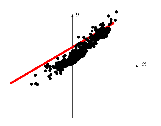
To find, or learn, a good hypothesis out of the infinite set \eqref{equ_def_linear_map_scalar}, we need to somehow assess the quality of a particular hypothesis map. ML methods use a loss function for this purpose. A loss function is used to quantify the difference between the actual data and the predictions obtained from a hypothesis map (see fig_scatterplot_temp_FMI_linalg). One widely-used example of a loss function is the squared error loss [math](\truelabel-h(\feature))^2[/math]. Using this loss function, ML methods learn a hypothesis map out of the model \eqref{equ_def_linear_map_scalar} by tuning [math]\weight_{1},\weight_{0}[/math] to minimize the average loss

[[math]](1/\samplesize) \sum_{\sampleidx=1}^{\samplesize} \big( \truelabel^{(\sampleidx)} - h\big(\feature^{(\sampleidx)} \big) \big)^{2}.[[/math]]

The above weather prediction is prototypical for many other ML applications. fig_AlexMLBP illustrates the typical workflow of a ML method. Starting from some initial guess, ML methods repeatedly improve their current hypothesis based on (new) observed data.

Using the current hypothesis, ML methods make predictions or forecasts about future observations. The discrepancy between the predictions and the actual observations, as measured using some loss function, is used to improve the hypothesis. Learning happens during improving the current hypothesis based on the discrepancy between its predictions and the actual observations.

ML methods must start with some initial guess or choice for a good hypothesis. This initial guess can be based on some prior knowledge or domain expertise . While the initial guess for a hypothesis might not be made explicit in some ML methods, each method must use such an initial guess. In our weather prediction application discussed above, we used the linear model \eqref{equ_initial_hypo_FMI} as the initial hypothesis.

Each dot represents a specific days that is characterized by its minimum daytime temperature [math]\feature[/math] and its maximum daytime temperature [math]\truelabel[/math]. We also depict a straight line representing a linear predictor map. A main principle of ML methods is to learn a predictor (or hypothesis) map with minimum discrepancy between predictor map and data points. Different ML methods use different types of predictor maps (hypothesis space) and loss functions to quantify the discrepancy between hypothesis and actual data points.

Relation to Other Fields

ML builds on concepts from several other scientific fields. Conversely, ML provides important tools for many other scientific fields.

Linear Algebra

Modern ML methods are computationally efficient methods to fit high-dimensional models to large amounts of data. The models underlying state-of-the-art ML methods can contain billions of tunable or learnable parameters. To make ML methods computationally efficient we need to use suitable representations for data and models.

Maybe the most widely used mathematical structure to represent data is the Euclidean space [math]\mathbb{R}^{\featuredim}[/math] with some dimension [math]\featuredim \in \naturalnumbers[/math] . The rich algebraic and geometric structure of [math]\mathbb{R}^{\featuredim}[/math] allows us to design of ML algorithms that can process vast amounts of data to quickly update a model (parameters). fig_euclideanspace_dim2 depicts the Euclidean space [math]\mathbb{R}^{\featuredim}[/math] for [math]\featuredim=2[/math], which is used to construct scatterplots.

The Euclidean space [math]\mathbb{R}^{2}[/math] is constituted by all vectors (or points) [math]\datapoint = \big(z_{1},z_{2}\big)^{T}[/math] (with [math]z_{1},z_{2} \in \mathbb{R}[/math]) together with the inner product [math]\datapoint^{T} \datapoint' = z_{1}z'_{1}+z_{2}z'_{2}[/math].

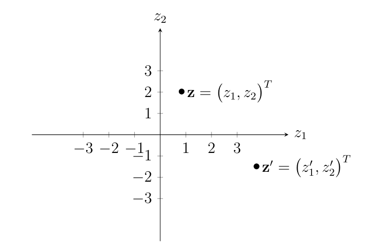
The scatterplot in fig_scatterplot_temp_FMI depicts data points (representing individual days) as vectors in the Euclidean space [math]\mathbb{R}^{2}[/math]. For a given data point, we obtain its associated vector [math]\datapoint=(\feature,\truelabel)^{T}[/math] in [math]\mathbb{R}^{2}[/math] by stacking the minimum daytime temperature [math]\feature[/math] and the maximum daytime temperature [math]\truelabel[/math] into the vector [math]\datapoint[/math] of length two.

We can use the Euclidean space [math]\mathbb{R}^{\featurelen}[/math] not only to represent data points but also to represent models for these data points. One such class of models is obtained by linear maps on [math]\mathbb{R}^{\featurelen}[/math]. fig_three_maps_example depicts some examples for such linear maps. We can then use the geometric structure of [math]\mathbb{R}^{\featurelen}[/math], defined by the Euclidean norm, to search for the best model. As an example, we could search for the linear model, represented by a straight line, such that the average (Euclidean) distance to the data points in fig_scatterplot_temp_FMI is as small as possible (see fig_scatterplot_temp_FMI_linalg). The properties of linear structures are studied within linear algebra . Some important ML methods, such as linear classifier (see Section Linear Regression ) or principal component analysis (PCA) (see Section Principal Component Analysis ) are direct applications of methods from linear algebra.

Optimization

A main design principle for ML methods is the formulation of ML problems as optimization problems . The weather prediction problem above can be formulated as the problem of optimizing (minimizing) the prediction error for the maximum daytime temperature. Many ML methods are obtained by straightforward applications of optimization methods to the optimization problem arising from a ML problem (or application).

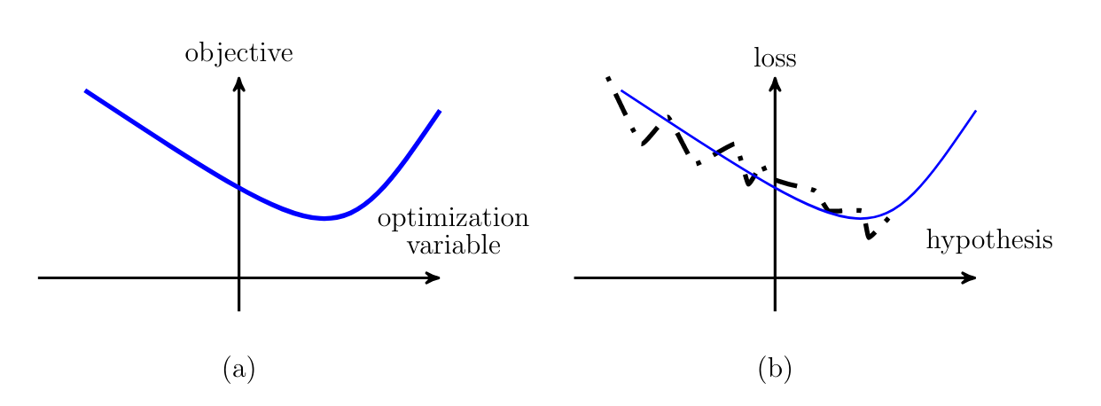
The statistical and computational properties of such ML methods can be studied using tools from the theory of optimization. What sets the optimization problems in ML apart from plain vanilla optimization problems (see fig_optml-(a)) is that we rarely have perfect access to the objective function to be minimized. ML methods learn a hypothesis by minimizing a noisy (or even incomplete) version (see fig_optml-(b)) of the ultimate objective function. The ultimate objective function for ML methods is often defined using an expectation over an unknown probability distribution for data points. Chapter Empirical Risk Minimization discusses methods that are based on estimating the objective function by empirical averages that are computed over a set of data points (which serve as a training set).

(a) A simple optimization problem consists of finding the values of an optimization variable that results in the minimum objective value. (b) ML methods learn (find) a hypothesis by minimizing a (average) loss. This average loss is a noisy version of the ultimate objective. This ultimate objective function is often defined as an expectation whose underlying probability distribution is unknown (see Section Empirical Risk ).

Theoretical Computer Science

Practical ML methods form a specific subclass of computing systems. Indeed, ML methods apply a sequence of computational operations to input data. The result of these computational operations are the predictions delivered to the user of the ML method. The interpretation of ML as computational systems allows to use tools from theoretical computer science to study the feasibility and intrinsic difficulty of ML problems. Even if a ML problem can be solved in theoretical sense, every practical ML method must fit the available computational infrastructure .

The available computational resources, such as processor time, memory and communication bandwidth, can vary significantly between different infrastructures. One example for such a computational infrastructure is a single desktop computer. Another example for a computational infrastructure is a cloud computing service which distributes data and computation over large networks of physical computers .

The focus of this book is on ML methods that can be understood as numerical optimization algorithms (see Chapter Empirical Risk Minimization and Gradient-Based Learning ). Most of these ML methods amount to (a large number of) matrix operations such as matrix multiplication or matrix inversion . Numerical linear algebra provides a vast algorithmic toolbox for the design of such ML methods . The recent success of ML methods in several application domains might be attributed to their efficient use of matrices to represent data and models. Using this representation allows us to implement the resulting ML methods using highly efficient hard- and software implementations for numerical linear algebra .

Information Theory

Information theory studies the problem of communication via noisy channels . fig_itml depicts the most simple communication problem that consists of an information source that wishes communicate a message [math]m[/math] over an imperfect (or noisy) channel to a receiver. The receiver tries to reconstruct (or learn) the original message based solely on the noisy channel output. Two main goals of information theory are (i) the characterization of conditions that allow reliable, i.e., nearly error-free, communication and (ii) the design of efficient transmitter (coding and modulation) and receiver (demodulation and decoding) methods.

It turns out that many concepts from information theory are very useful for the analysis and design of ML methods. As a point in case, Chapter Transparent and Explainable ML discusses the application of information-theoretic concepts to the design of explainable ML methods. On a more fundamental level, we can identify two core communication problems that arise within ML. These communication problems correspond, respectively, to the inference (making a prediction) and the learning (adjusting or improving the current hypothesis) step of a ML method (see fig_AlexMLBP).

We can an interpret the inference step of ML as the problem of decoding the true label of a data point for which we only know its features. This communication problem is depicted in fig_itml-(b). Here the message to be communicated is the true label of a random data point. This data point is communicated over a channel that only passes through its features. The inference step within a ML method then tries to decode the original message (true label) from the channel output (features) resulting in the predicted label. A recent line of work used this communication problem to study deep learning methods .

(a) A basic communication system involves an information source that emits a message [math]m[/math]. The message is processed by some transmitter and passed through a noisy channel. The receiver tries to recover the original message [math]m[/math] by computing the decoded message [math]\hat{m}[/math]. (b) The inference step of ML (see fig_AlexMLBP) corresponds to a communication problem with an information source emitting a data point with features [math]\featurevec[/math] and label [math]\truelabel[/math]. The ML method receives the features [math]\featurevec[/math] and, in an effort to recover the true label [math]\truelabel[/math], computes the predicted label [math]\hat{\truelabel}[/math]. (c) The learning or adaptation step of ML (see fig_AlexMLBP) solves a communication problem with some source that selects a true (but unknown) hypothesis [math]h^{*}[/math] as the message. The message is passed through an abstract channel that outputs a set [math]\dataset[/math] of labeled data points which are used as the training set by an ML method. The ML method tries to decode the true hypothesis resulting in the learnt the hypothesis [math]\hat{h}[/math].

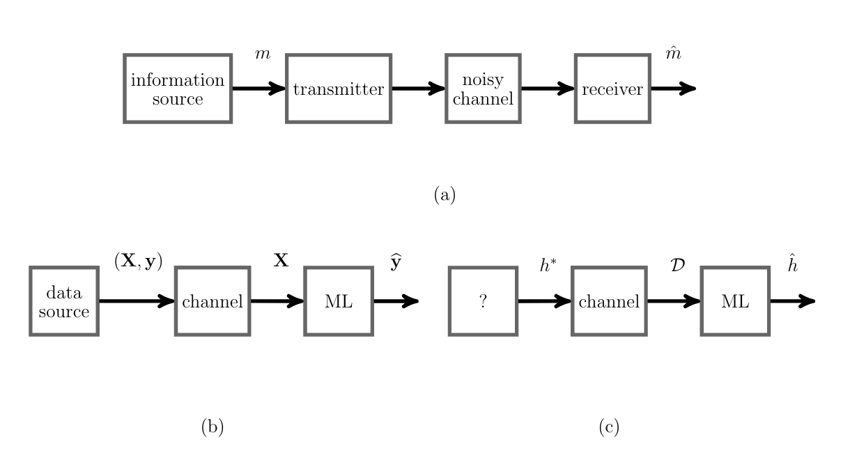
A second core communication problem of ML corresponds to the problem of learning (or adjusting) a hypothesis (see fig_itml-(c)). In this problem, the source selects some true hypothesis as message. This message is then communicated to an abstract channel that models the data generation process. The output of this abstract channel are data points in a training set [math]\dataset[/math] (see Chapter Empirical Risk Minimization ). The learning step of a ML method, such as empirical risk minimization (ERM) of Chapter Empirical Risk Minimization , then amounts to the decoding of the message (true hypothesis) based on the channel output (training set). There is significant line or research that uses the communication problem in fig_itml-(c) to characterize the fundamental limits of ML problems and methods such as the minimum required number of training data points that makes learning feasible .

The relevance of information theoretic concepts and methods for ML is boosted by the recent trend towards distributed or federated ML . We can interpret federated learning (FL) applications as a specific type of network communication problems . In particular, we can apply network coding techniques to the design and analysis of FL methods .

Probability Theory and Statistics

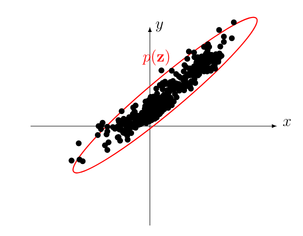
Consider the data points [math]\rawfeaturevec^{(1)},\ldots,\rawfeaturevec^{(\samplesize)}[/math] depicted in fig_scatterplot_temp_FMI. Each data point represents some previous day that is characterized by its minimum and maximum daytime temperature as measured at a specific FMI weather observation station. It might be useful to interpret these data points as realizations of independent and identically distributed (iid) random variable (RV)s with common (but typically unknown) probability distribution [math]\prob{\datapoint}[/math]. fig_scatterplot_temp_FMI_stat_model extends the scatterplot in fig_scatterplot_temp_FMI by adding a contour line of the underlying probability distribution [math]\prob{\rawfeaturevec}[/math] .

Probability theory offers principled methods for estimating a probability distribution from a set of data points (see Section Maximum Likelihood ). Let us assume we know (an estimate of) the (joint) probability distribution [math]\prob{\datapoint}[/math] of features and label of a data point [math]\datapoint=\big(\featurevec,\truelabel)[/math]. A principled approach to predict the label value of a data point with features [math]\featurevec[/math] is based on evaluating the conditional probability distribution [math]\prob{\truelabel=\hat{\truelabel}|\featurevec}[/math]. The conditional probability distribution [math]\prob{\hat{\truelabel}=\truelabel|\featurevec}[/math] quantifies how likely it is that [math]\hat{\truelabel}[/math] is the actual label value of a data point. We can evaluate the quantity [math]\prob{\hat{\truelabel}=\truelabel|\featurevec}[/math] for any candidate value [math]\hat{\truelabel}[/math] as soon as we know the features [math]\featurevec[/math] of this data point.

Depending on the performance criterion or loss function, the optimal prediction [math]\hat{\truelabel}[/math] is either given by the mode of [math]\prob{\hat{\truelabel}=\truelabel|\featurevec}[/math] its mean or some other characteristic value. It is important to note that this probabilistic approach not only provides a specific prediction (point-estimate) but an entire distribution [math]\prob{\hat{\truelabel}=\truelabel|\featurevec}[/math] over possible predictions. This distribution allows to construct confidence measures, such as the variance, that can be provided along with the prediction.

Having a probabilistic model, in the form of a probability distribution [math]\prob{\datapoint}[/math], for the data arising in an ML application not only allows us to compute predictions for labels of data points. We can also use [math]\prob{\datapoint}[/math] to augment the available dataset by randomly drawing (generating) new data points from [math]\prob{\datapoint}[/math] (see Section Data Augmentation).

ML methods that rely on a probabilistic model for data are sometimes referred to as generative methods. A recently popularized class of generative methods, that uses models obtained from artificial neural network (ANN), is known as generative adversarial networks .

Each dot represents a data point [math]\datapoint=\big(\feature,\truelabel\big)[/math] that is characterized by a numeric feature [math]\feature[/math] and a numeric label [math]\truelabel[/math]. We also indicate a contour-line of a probability distribution [math]\prob{\datapoint}[/math] that could be used to interpret data points as realizations of iid RVs with common probability distribution [math]\prob{\datapoint}[/math].

Artificial Intelligence

ML theory and methods are instrumental for the analysis and design of artificial intelligence (AI) . An AI system, typically referred to as an agent, interacts with its environment by executing (choosing between different) actions. These actions influence the environment as well as the state of the AI agent. The behaviour of an AI system is determined by how the perceptions made about the environment are used to form the next action.

From an engineering point of view, AI aims at optimizing behaviour to maximize a long-term return. The optimization of behaviour is based solely on the perceptions made by the agent. Let us consider some application domains where AI systems can be used:

Application	Description
forest fire management system	perceptions given by satellite images and local observations using sensors or “crowd sensing” via some mobile application which allows humans to notify about relevant events; actions amount to issuing warnings and bans of open fire; return is the reduction of number of forest fires.
control unit for combustion engines	perceptions given by various measurements such as temperature, fuel consistency; actions amount to varying fuel feed and timing and the amount of recycled exhaust gas; return is measured in reduction of emissions.
severe weather warning service	perceptions given by weather radar; actions are preventive measures taken by farmers or power grid operators; return is measured by savings in damage costs (see [1])
automated benefit application system for the Finnish social insurance institute (Kela)	perceptions given by information about application and applicant; actions are either to accept or to reject the application along with a justification for the decision; return is measured in reduction of processing time (applicants tend to prefer getting decisions quickly)
personal diet assistant	perceived environment is the food preferences of the app user and their health condition; actions amount to personalized suggestions for healthy and tasty food; return is the increase in well-being or the reduction in public spending for health-care.
Rumba	the cleaning robot Rumba (see Figure fig:cleaning_robot) perceives its environment using different sensors (distance sensors, on-board camera); actions amount to choosing different moving directions (north, south, east, west); return might be the amount of cleaned floor area within a particular time period.
personal health assistant	perceptions given by current health condition (blood values, weight,...), lifestyle (preferred food, exercise plan); actions amount to personalized suggestions for changing lifestyle habits (less meat, more walking,...); return is measured via the level of well-being (or the reduction in public spending for health-care).
government-system for a country	perceived environment is constituted by current economic and demographic indicators such as unemployment rate, budget deficit, age distribution,...; actions involve the design of tax and employment laws, public investment in infrastructure, organization of health-care system; return might be determined by the gross domestic product, the budget deficit or the gross national happiness (cf. gross national happiness).

A cleaning robot chooses actions (moving directions) to maximize a long-term reward measured by the amount of cleaned floor area per day.

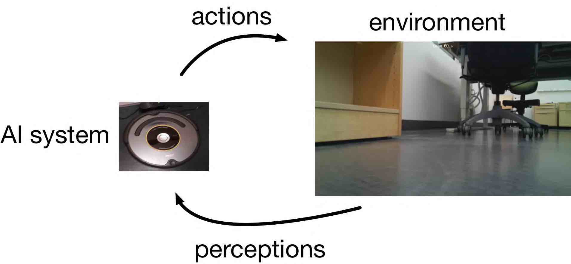
ML methods are used on different levels by an AI agent. On a lower level, ML methods help to extract the relevant information from raw data. ML methods are used to classify images into different categories which are then used an input for higher level functions of the AI agent.

ML methods are also used for higher level tasks of an AI agent. To behave optimally, an agent is required to learn a good hypothesis for how its behaviour affects its environment. We can think of optimal behaviour as a consequent choice of actions that might be predicted by ML methods.

What sets AI applications apart from more traditional ML application is that there is an strong interaction between ML method and the data generation process. Indeed, AI agents use the predictions of an ML method to select its next action which, in turn, influences the environment which generates new data points. The ML subfield of active learning studies methods that can influence the data generation .

Another characteristic of AI applications is that they typically allow ML methods to evaluate the quality of a hypothesis only in hindsight. Within a basic (supervised) ML application it is possible for a ML method to try out many different hypotheses on the same data point. These different hypotheses are then scored by their discrepancies with a known correct predictions. In contrast to such passive ML applications, AI applications involve data points for which it is infeasible to determine the correct predictions.

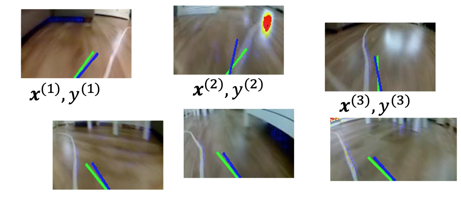
Let us illustrate the above differences between ML and AI applications with the help of a self-driving toy car. The toy-car is equipped with a small onboard computer, camera, sensors and actors that allow to define the steering direction. Our goal is to program the onboard computer such that it implements an AI agent that optimally steers the toy-car. This AI application involves data points that represent the different (temporal) states of the toy car during its ride. We use a ML method to predict the optimal steering direction for the current state. The prediction for the optimal steering angle is obtained by a hypothesis map that reads a snapshot form an on-board camera. Since these predictions are used to actually steer the car, they influence the future data points (states) that will be obtained.

Note that we typically do not know the actual optimal steering direction for each possible state of the car. It is infeasible to let the toy car roam around along any possible path and then manually label each on-board camera snapshot with the optimal steering direction (see fig_rl_donkey). The usefulness of a prediction can be measured only in an indirect fashion by using some form of reward signal. Such a reward signal could be obtained from a distance sensor that allows to determine if the toy car reduced the distance to a target location.

Flavours of Machine Learning

ML methods read in data points which are generated within some application domain. An individual data point is characterized by various properties. We find it convenient to divide the properties of data points into two groups: features and labels (see Section The Data ). Features are properties that we measure or compute easily in an automated fashion. Labels are properties that cannot be measured easily and often represent some higher level fact (or quantity of interest) whose discovery often requires human experts.

Roughly speaking, ML aims at learning to predict (approximating or guessing) the label of a data point based solely on the features of this data point. Formally, the prediction is obtained as the function value of a hypothesis map whose input argument are the features of a data point. Since any ML method must be implemented with finite computational resources, it can only consider a subset of all possible hypothesis maps. This subset is referred to as the hypothesis space or model underlying a ML method. Based on how ML methods assess the quality of different hypothesis maps we distinguish three main flavours of ML: supervised, unsupervised and reinforcement learning.

Supervised Learning

The main focus of this book is on supervised ML methods. These methods use a training set that consists of labeled data points (for which we know the correct label values). We refer to a data point as labeled if its label value is known. Labeled data points might be obtained from human experts that annotate (label) data points with their label values. There are marketplaces for renting human labelling workforce . Supervised ML searches for a hypothesis that can imitate the human annotator and allows to predict the label solely from the features of a data point.

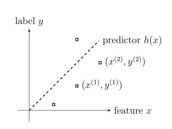
fig_curve_fitting illustrates the basic principle of supervised ML methods. These methods learn a hypothesis with minimum discrepancy between its predictions and the true labels of the data points in the training set. Loosely speaking, supervised ML fits a curve (the graph of the predictor map) to labeled data points in a training set. For the actual implementing of this curve fitting we need a loss function that quantifies the fitting error. Supervised ML method differ in their choice for a loss function to measure the discrepancy between predicted label and true label of a data point.

While the principle behind supervised ML sounds trivial, the challenge of modern ML applications is the sheer amount of data points and their complexity. ML methods must process billions of data points with each single data points characterized by a potentially vast number of features. Consider data points representing social network users, whose features include all media that has been posted (videos, images, text). Besides the size and complexity of datasets, another challenge for modern ML methods is that they must be able to fit highly non-linear predictor maps. Deep learning methods address this challenge by using a computationally convenient representation of non-linear maps via artificial neural networks .

Supervised ML methods fit a curve to a set of data points (which serve as a training set). The curve represents a hypothesis out of some hypothesis space or model. The fitting error (or training error) is measured using a loss function. Different ML methods use different combinations of model and loss function.

Unsupervised Learning

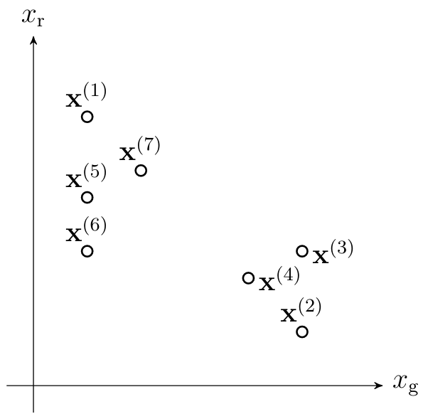
Some ML methods do not require knowing the label value of any data point and are therefore referred to as unsupervised ML methods. Unsupervised methods must rely solely on the intrinsic structure of data points to learn a good hypothesis. Thus, unsupervised methods do not need a teacher or domain expert who provides labels for data points (used to form a training set). Chapters Clustering and Feature Learning discuss two large families of unsupervised methods, referred to as clustering and feature learning methods.

Clustering methods group data points into few subsets or cluster. The data points within the same cluster should be more similar with each other than with data points outside the cluster (see fig_unsupervised_clustering). Feature learning methods determine numeric features such that data points can be processed efficiently using these features. Two important applications of feature learning are dimensionality reduction and data visualization.

Clustering methods learn to predict the cluster (or group) assignments of data points based solely on their features. Chapter Clustering discusses clustering methods that are unsupervised in the sense of not requiring the knowledge of the true cluster assignment of any data point.

Reinforcement Learning

In general, ML methods use a loss function to evaluate and compare different hypotheses. The loss function assigns a (typically non-negative) loss value to a pair of a data point and a hypothesis. ML methods search for a hypothesis, out of (typically large) hypothesis space, that incurs minimum loss for any data point. Reinforcement learning (RL) studies applications where the predictions obtained by a hypothesis influences the generation of future data points. RL applications involve data points that represent the states of a programmable system (an AI agent) at different time instants. The label of such a data point has the meaning of an optimal action that the agent should take in a given state. Similar to unsupervised ML, RL methods often must learn a hypothesis without having access to any labeled data point.

In stark contrast to supervised and unsupervised ML methods, RL methods cannot evaluate the loss function for different choices of a hypothesis. Consider a RL method that has to predict the optimal steering angle of a car. Naturally, we can only evaluate the usefulness specific combination of predicted label (steering angle) and the current state of the car. It is impossible to try out two different hypotheses at the same time as the car cannot follow two different steering angles (obtained by the two hypotheses) at the same time.

Mathematically speaking, RL methods can evaluate the loss function only point-wise for the current hypothesis that has been used to obtain the most recent prediction. These point-wise evaluations of the loss function are typically implemented by using some reward signal . Such a reward signal might be obtained from a sensing device and allows to quantify the usefulness of the current hypothesis.

One important application domain for RL methods is autonomous driving (see fig_rl_donkey). Consider data points that represent individual time instants [math]\timeidx=0,1,\ldots[/math] during a car ride. The features of the [math]\timeidx[/math]th data point are the pixel intensities of an on-board camera snapshot taken at time [math]\timeidx[/math]. The label of this data point is the optimal steering direction at time [math]\timeidx[/math] to maximize the distance between the car and any obstacle. We could use a ML method to learn hypothesis for predicting the optimal steering direction solely from the pixel intensities in the on-board camera snapshot. The loss incurred by a particular hypothesis is determined from the measurement of a distance sensor after the car moved along the predicted direction. We can evaluate the loss only for the hypothesis that has actually been used to predict the optimal steering direction. It is impossible to evaluate the loss for other predictions of the optimal steering direction since the car already moved on.

Autonomous driving requires to predict the optimal steering direction (label) based on an on-board camera snapshot (features) in each time instant. RL methods sequentially adjust a hypothesis for predicting the steering direction from the snapshot. The quality of the current hypothesis is evaluated by the measurement of a distance sensor (to avoid collisions with obstacles).

Organization of this Book

Chapter Three Components of ML introduces the notions of data, a model and a loss function as the three main components of ML. We will also highlight some of the computational and statistical aspects that might guide the design choices arising for these three components. A guiding theme of this book is the depiction of ML methods as combinations of specific design choices for data representation, the model and the loss function. Put differently, we aim at mapping out the vast landscape of ML methods in an abstract three-dimensional space spanned by the three dimensions: data, model and loss.

Chapter The Landscape of ML details how several well-known ML methods are obtained by specific design choices for data (representation), model and loss function. Examples range from basic linear regression (see Section Linear Regression ) via support vector machine (SVM) (see Section Support Vector Machines ) to deep reinforcement learning (see Section Deep Reinforcement Learning ).

Chapter Empirical Risk Minimization discusses a principle approach to combine the three components within a practical ML method. In particular, Chapter Empirical Risk Minimization explains how a simple probabilistic model for data lends naturally to the principle of ERM. This principle translates the problem of learning into an optimization problem. ML methods based on the ERM are therefore a special class of optimization methods. The ERM principle can be interpreted as a precise mathematical formulation of the learning by trial and error paradigm.

Chapter Gradient-Based Learning discusses a family of iterative methods for solving the ERM problem introduced in Chapter Empirical Risk Minimization . These methods use the concept of a gradient to locally approximate the objective function used in ERM. Gradient-based methods are widely used within deep learning methods to learn useful weights for large ANN (see Section Deep Learning and ).

The ERM principle of Chapter Empirical Risk Minimization requires a hypothesis to accurately predict the labels of data points in a training set. However, the ultimate goal of ML is to learn a hypothesis that delivers accurate predications for any data point and not only the training set. Chapter Model Validation and Selection discusses some basic validation techniques that allow to probe a hypothesis outside the training set that has been used to learn (optimize) this hypothesis via ERM. Validation techniques are instrumental for model selection, i.e., to choose the best model from a given set of candidate models. Chapter Regularization presents regularization techniques that aim at replacing the training error of a candidate hypothesis with an estimate (or approximation) of its average loss incurred for data points outside the training set.

The focus of Chapters The Landscape of ML - Regularization is on supervised ML methods that require a training set of labeled data points. Chapters Clustering and Feature Learning are devoted to unsupervised ML methods which do not require any labeled data. Chapter Clustering discusses clustering methods that partition data points into coherent groups which are referred to as clusters. Chapter Feature Learning discusses methods that automatically determine the most relevant characteristics (or features) of a data point. This chapter also highlights the importance of using only the most relevant features of a data point, and to avoid irrelevant features, to reduce computational complexity and improve the accuracy of ML methods (such as those discussed in Chapter The Landscape of ML ).

The success of ML methods becomes increasingly dependent on their explainability or transparency for the user of the ML method . The explainability of a ML method and its predictions typically depends on the background knowledge of the user which might vary significantly. Chapter Transparent and Explainable ML discusses two different approaches to obtain personalized explainable ML. These techniques use a feedback signal, which is provided for the data points in a training set, to either compute personalized explanations for a given ML method or to choose models that are intrinsically explainable to a specific user.

Prerequisites. We assume familiarity with basic notions and concepts of linear algebra, real analysis, and probability theory . For a brief review of those concepts, we recommend and the references therein. A main goal of this book is to develop the basic ideas and principles behind ML methods using a minimum of probability theory. However, some rudimentary knowledge about the concept of expectations, probability density function of a continuous (real-valued) RV and probability mass function of a discrete RV is helpful .

General References

Jung, Alexander (2022). Machine Learning: The Basics. Signapore: Springer. doi:10.1007/978-981-16-8193-6.

Jung, Alexander (2022). "Machine Learning: The Basics". arXiv:1805.05052.

References

- T. Mitchell. The need for biases in learning generalizations. Technical Report CBM-TR 5-110,, Rutgers University, New Brunswick, New Jersey, USA, 1980
- 2.0 2.1 W. Rudin. Principles of Mathematical Analysis McGraw-Hill, New York, 3 edition, 1976
- 3.0 3.1 3.2 G. Strang. Introduction to Linear Algebra Wellesley-Cambridge Press, MA, 5 edition, 2016
- S. Sra, S. Nowozin, and S. J. Wright, editors. Optimization for Machine Learning MIT Press, 2012
- L. Pitt and L. G. Valiant. Computational limitations on learning from examples. J. ACM 35(4):965--984, Oct. 1988
- L. G. Valiant. A theory of the learnable. In Proceedings of the Sixteenth Annual ACM Symposium on Theory of Computing STOC '84, pages 436--445, New York, NY, USA, 1984. Association for Computing Machinery
- C. Millard, editor. Cloud Computing Law Oxford University Press, 2 edition, May 2021
- G. H. Golub and C. F. Van Loan. Matrix Computations Johns Hopkins University Press, Baltimore, MD, 3rd edition, 1996
- G. Strang. Computational Science and Engineering Wellesley-Cambridge Press, MA, 2007
- 10.0 10.1 10.2 10.3 I. Goodfellow, Y. Bengio, and A. Courville. Deep Learning MIT Press, 2016
- 11.0 11.1 N. Tishby and N. Zaslavsky. Deep learning and the information bottleneck principle. In 2015 IEEE Information Theory Workshop (ITW) pages 1--5, 2015
- C. E. Shannon. Communication in the presence of noise. 1948
- T. M. Cover and J. A. Thomas. Elements of Information Theory Wiley, New Jersey, 2 edition, 2006
- 14.0 14.1 14.2 A. E. Gamal and Y.-H. Kim. Network Information Theory Cambridge Univ. Press, 2012
- W. Wang, M. J. Wainwright, and K. Ramchandran. Information-theoretic bounds on model selection for Gaussian Markov random fields. In Proc. IEEE ISIT-2010 pages 1373--1377, Austin, TX, Jun. 2010
- M. J. Wainwright. Information-theoretic limits on sparsity recovery in the high-dimensional and noisy setting. IEEE Trans. Inf. Theory 55(12):5728--5741, Dec. 2009
- N. P. Santhanam and M. J. Wainwright. Information-theoretic limits of selecting binary graphical models in high dimensions. IEEE Trans. Inf. Theory 58(7):4117--4134, Jul. 2012
- N. Tran, O. Abramenko, and A. Jung. On the sample complexity of graphical model selection from non-stationary samples. IEEE Transactions on Signal Processing 68:17--32, 2020
- A. Jung, Y. Eldar, and N. Görtz. On the minimax risk of dictionary learning. IEEE Trans. Inf. Theory 62(3):1501 -- 1515, Mar. 2016
- B. McMahan, E. Moore, D. Ramage, S. Hampson, and B. A. y Arcas. Communication-efficient learning of deep networks from decentralized data. In A. Singh and J. Zhu, editors, Proceedings of the 20th International Conference on Artificial Intelligence and Statistics volume 54 of Proceedings of Machine Learning Research pages 1273--1282, Fort Lauderdale, FL, USA, 20--22 Apr 2017. PMLR
- V. Smith, C.-K. Chiang, M. Sanjabi, and A. Talwalkar. Federated multi-task learning. In Advances in Neural Information Processing Systems volume 30, 2017
- F. Sattler, K. Müller, and W. Samek. Clustered federated learning: Model-agnostic distributed multitask optimization under privacy constraints. IEEE Transactions on Neural Networks and Learning Systems 2020
- Y. SarcheshmehPour, M. Leinonen, and A. Jung. Federated learning from big data over networks. In Proc. IEEE Int. Conf. on Acoustics, Speech and Signal Processing (ICASSP), preprint: https://arxiv.org/pdf/2010.14159.pdf 2021
- 24.0 24.1 D. Bertsekas and J. Tsitsiklis. Introduction to Probability Athena Scientific, 2 edition, 2008
- I. J. Goodfellow, J. Pouget-Abadie, M. Mirza, B. Xu, D. Warde-Farley, S. Ozair, A. Courville, and Y. Bengio. Generative adversarial nets. In Proc. Neural Inf. Proc. Syst. (NIPS) 2014
- S. J. Russel and P. Norvig. Artificial Intelligence - A Modern Approach Prentice Hall, New York, 3 edition, 2010
- D. Cohn, Z. Ghahramani, and M. Jordan. Active learning with statistical models. J. Artif. Int. Res. 4(1):129--145, March 1996
- A. Sorokin and D. Forsyth. Utility data annotation with amazon mechanical turk. In 2008 IEEE Computer Society Conference on Computer Vision and Pattern Recognition Workshops pages 1--8, 2008
- R. Sutton and A. Barto. Reinforcement learning: An introduction MIT press, Cambridge, MA, 2 edition, 2018
- H. Hagras. Toward human-understandable, explainable ai. Computer 51(9):28--36, Sep. 2018
- J. McInerney, B. Lacker, S. Hansen, K. Higley, H. Bouchard, A. Gruson, and R. Mehrotra. Explore, exploit, and explain: personalizing explainable recommendations with bandits. In Proceedings of the 12th ACM Conference on Recommender Systems 2018
- R. Gray. Probability, Random Processes, and Ergodic Properties Springer, New York, 2 edition, 2009