guide:7d6298862b

[math] \require{textmacros} \def \bbeta {\bf \beta} \def\fat#1{\mbox{\boldmath$#1$}} \def\reminder#1{\marginpar{\rule[0pt]{1mm}{11pt}}\textbf{#1}} \def\SSigma{\bf \Sigma} \def\ttheta{\bf \theta} \def\aalpha{\bf \alpha} \def\bbeta{\bf \beta} \def\ddelta{\bf \delta} \def\eeta{\bf \eta} \def\llambda{\bf \lambda} \def\ggamma{\bf \gamma} \def\nnu{\bf \nu} \def\vvarepsilon{\bf \varepsilon} \def\mmu{\bf \mu} \def\nnu{\bf \nu} \def\ttau{\bf \tau} \def\SSigma{\bf \Sigma} \def\TTheta{\bf \Theta} \def\XXi{\bf \Xi} \def\PPi{\bf \Pi} \def\GGamma{\bf \Gamma} \def\DDelta{\bf \Delta} \def\ssigma{\bf \sigma} \def\UUpsilon{\bf \Upsilon} \def\PPsi{\bf \Psi} \def\PPhi{\bf \Phi} \def\LLambda{\bf \Lambda} \def\OOmega{\bf \Omega} [/math]

Constrained estimation

The ad-hoc fix of to super-collinearity of the design matrix (and, consequently the singularity of the matrix [math]\mathbf{X}^{\top} \mathbf{X}[/math]) has been motivated post-hoc. The ridge regression estimator minimizes the ridge loss function, which is defined as:

[[math]] \begin{eqnarray} \mathcal{L}_{\mbox{{\tiny ridge}}}(\bbeta; \lambda) & = & \| \mathbf{Y} - \mathbf{X} \bbeta \|^2_2 + \lambda \| \bbeta \|^2_2 \, \, \, = \, \, \, \sum\nolimits_{i=1}^n (Y_i - \mathbf{X}_{i\ast} \bbeta)^2 + \lambda \sum\nolimits_{j=1}^p \beta_j^2. \label{form.ridgeLossFunction} \end{eqnarray} [[/math]]

This loss function is the traditional sum-of-squares augmented with a penalty. The particular form of the penalty, [math]\lambda \| \bbeta \|^2_2[/math] is referred to as the ridge penalty and [math]\lambda[/math] as the penalty parameter. For [math]\lambda=0[/math], minimization of the ridge loss function yields the ML estimator (if it exists). For any [math]\lambda \gt 0[/math], the ridge penalty contributes to the loss function, affecting its minimum and its location. The minimum of the sum-of-squares is well-known. The minimum of the ridge penalty is attained at [math]\bbeta = \mathbf{0}_{p}[/math] whenever [math]\lambda \gt 0[/math]. The [math]\bbeta[/math] that minimizes [math]\mathcal{L}_{\mbox{{\tiny ridge}}}(\bbeta; \lambda)[/math] then balances the sum-of-squares and the penalty. The effect of the penalty in this balancing act is to shrink the regression coefficients towards zero, its minimum. In particular, the larger [math]\lambda[/math], the larger the contribution of the penalty to the loss function, the stronger the tendency to shrink non-zero regression coefficients to zero (and decrease the contribution of the penalty to the loss function). This motivates the name ‘penalty’ as non-zero elements of [math]\bbeta[/math] increase (or penalize) the loss function.

To verify that the ridge regression estimator indeed minimizes the ridge loss function, proceed as usual. Take the derivative with respect to [math]\bbeta[/math]:

[[math]] \begin{eqnarray*} \frac{\partial}{\partial \bbeta} \mathcal{L}_{\mbox{{\tiny ridge}}}(\bbeta; \lambda) & = & -2 \mathbf{X}^{\top} (\mathbf{Y} - \mathbf{X} \bbeta) + 2 \lambda \mathbf{I}_{pp} \bbeta \, \, \, = \, \, \, -2 \mathbf{X}^{\top} \mathbf{Y} + 2 ( \mathbf{X}^{\top} \mathbf{X} + \lambda \mathbf{I}_{pp}) \bbeta. \end{eqnarray*} [[/math]]

Equate the derivative to zero and solve for [math]\bbeta[/math]. This yields the ridge regression estimator.

The ridge estimator is thus a stationary point of the ridge loss function. A stationary point corresponds to a minimum if the Hessian matrix with second order partial derivatives is positive definite. The Hessian of the ridge loss function is

[[math]] \begin{eqnarray*} \frac{\partial^2}{\partial \bbeta \, \partial \bbeta^{\top}} \mathcal{L}_{\mbox{{\tiny ridge}}}(\bbeta; \lambda) & = & 2 ( \mathbf{X}^{\top} \mathbf{X} + \lambda \mathbf{I}_{pp}). \end{eqnarray*} [[/math]]

This Hessian is the sum of the (semi-)positive definite matrix [math]\mathbf{X}^{\top} \mathbf{X}[/math] and the positive definite matrix [math]\lambda \, \mathbf{I}_{pp}[/math]. Lemma 14.2.4 of then states that the sum of these matrices is itself a positive definite matrix. Hence, the Hessian is positive definite and the ridge loss function has a stationary point at the ridge estimator, which is a minimum.

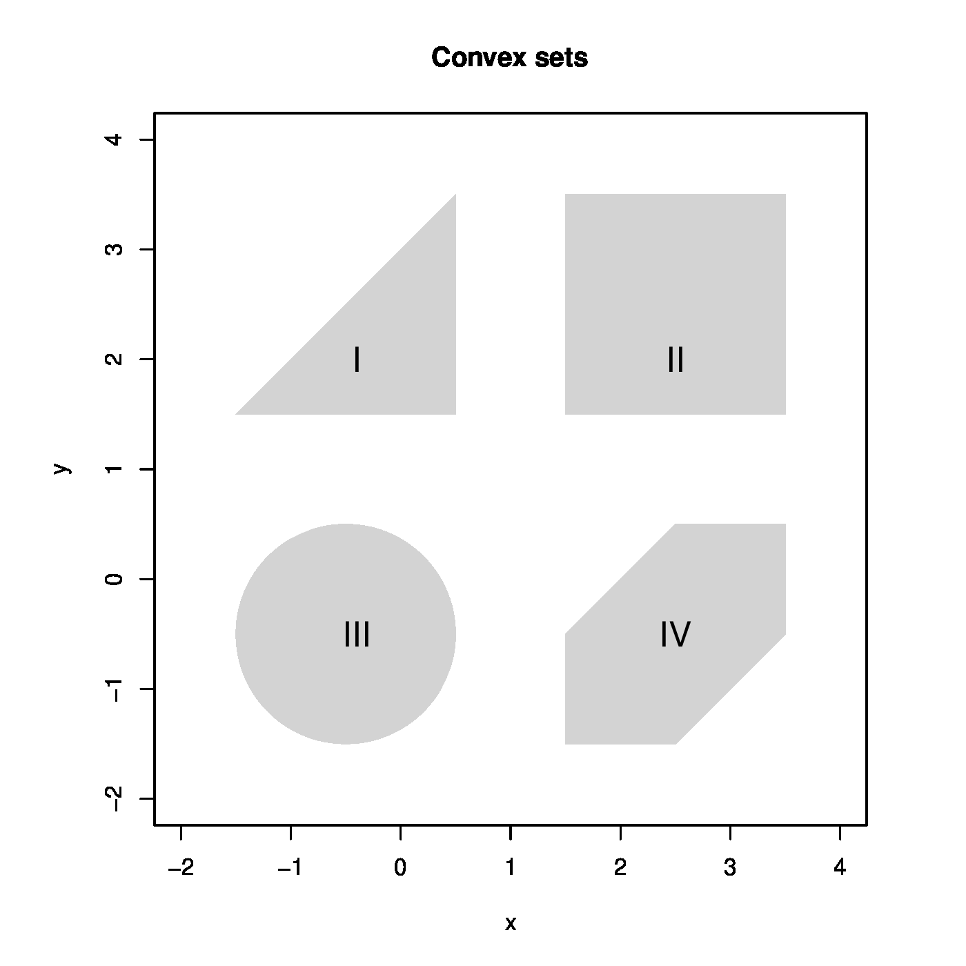
The ridge regression estimator minimizes the ridge loss function. It rests to verify that it is a global minimum. To this end we introduce the concept of a convex function. As a prerequisite, a set [math]\mathcal{S} \subset \mathbb{R}^p[/math] is called convex if for all [math]\bbeta_1, \bbeta_2 \in \mathcal{S}[/math] their weighted average [math]\bbeta_{\theta} = (1 - \theta) \bbeta_1 + \theta \bbeta_2[/math] for all [math]\theta \in [0, 1][/math] is itself an element of [math]\mathcal{S}[/math], thus [math]\bbeta_{\theta} \in \mathcal{S}[/math]. If for all [math]\theta \in (0, 1)[/math], the weighted average [math]\bbeta_{\theta}[/math] is inside [math]\mathcal{S}[/math] and not on its boundary, the set is called strictly convex. Examples of (strictly) convex and nonconvex sets are depicted in Figure. A function [math]f(\cdot)[/math] is (strictly) convex if the set [math]\{ y \, : \, y \geq f(\bbeta) \mbox{ for all } \bbeta \in \mathcal{S} \mbox{ for any convex } \mathcal{S} \}[/math], called the epigraph of [math]f(\cdot)[/math], is (strictly) convex. Examples of (strictly) convex and nonconvex functions are depicted in Figure. The ridge loss function is the sum of two parabola's: one is at least convex and the other strictly convex in [math]\bbeta[/math]. The sum of a convex and strictly convex function is itself strictly convex (see Lemma 9.4.2 of ). The ridge loss function is thus strictly convex. Theorem 9.4.1 of then warrants, by the strict convexity of the ridge loss function, that the ridge regression estimator is a global minimum.

From the ridge loss function the limiting behavior of the variance of the ridge regression estimator can be understood. The ridge penalty with its minimum [math]\bbeta = \mathbf{0}_{p}[/math] does not involve data and, consequently, the variance of its minimum equals zero. With the ridge regression estimator being a compromise between the maximum likelihood estimator and the minimum of the penalty, so is its variance a compromise of their variances. As [math]\lambda[/math] tends to infinity, the ridge regression estimator and its variance converge to the minimizer of the loss function and the variance of the minimizer, respectively. Hence, in the limit (large [math]\lambda[/math]) the variance of the ridge regression estimator vanishes. Understandably, as the penalty now fully dominates the loss function and, consequently, it does no longer involve data (i.e. randomness).

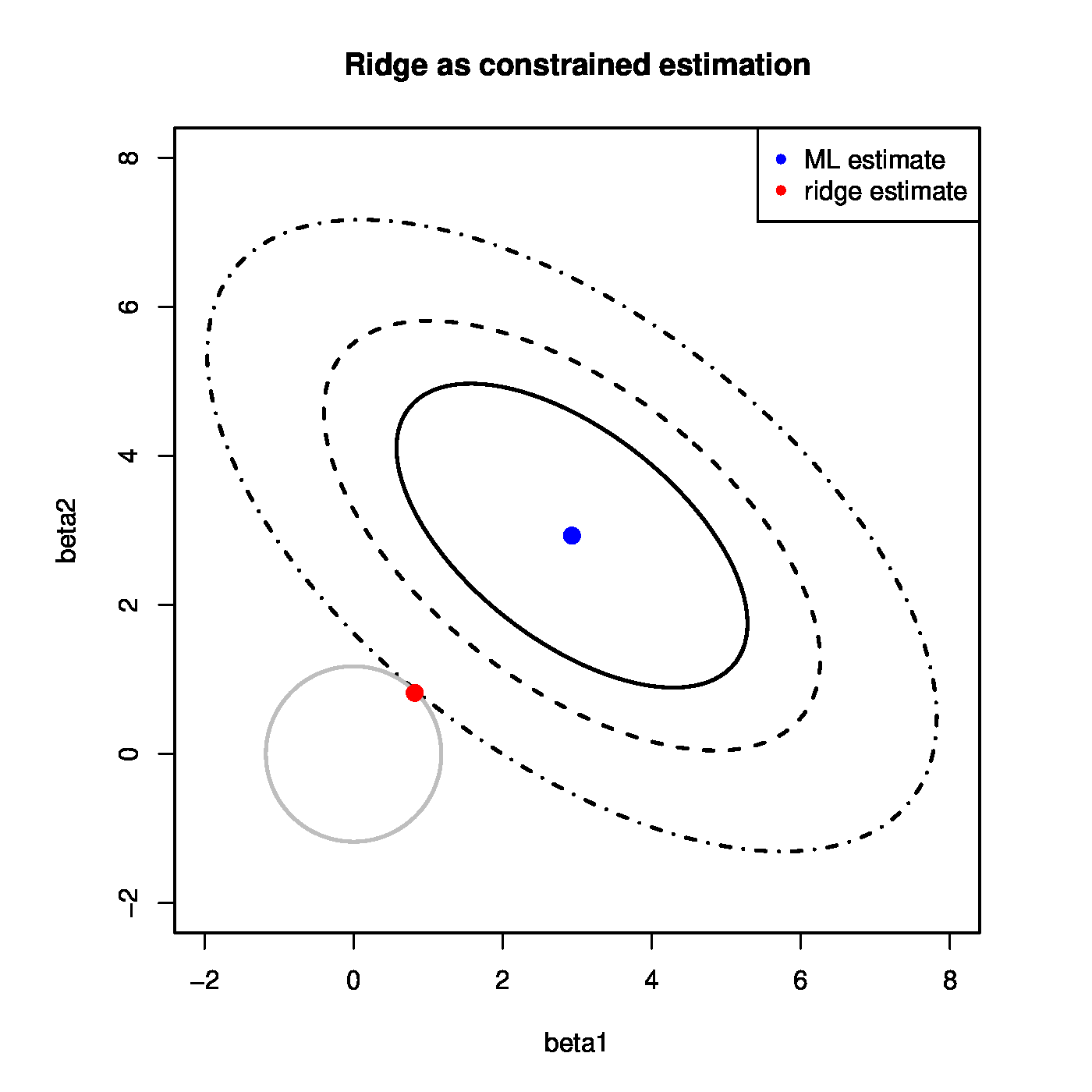
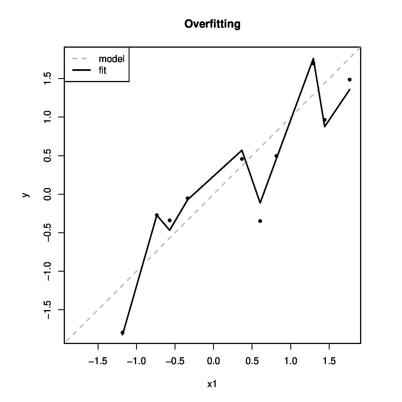
Figure: Top panels show examples of convex (left) and nonconvex (right) sets. Middle panels show examples of convex (left) and nonconvex (right) functions. The left bottom panel illustrates the ridge estimation as a constrained estimation problem. The ellipses represent the contours of the ML loss function, with the blue dot at the center the ML estimate. The circle is the ridge parameter constraint. The red dot is the ridge estimate. It is at the intersection of the ridge constraint and the smallest contour with a non-empty intersection with the constraint. The right bottom panel shows the data corresponding to Example. The grey line represents the ‘true’ relationship, while the black line the fitted one.

Above it has been shown that the ridge estimator can be defined as:

[[math]] \begin{eqnarray} \label{form.ridgeEstViaPenEst} \hat{\bbeta}(\lambda) & = & \arg \min_{\bbeta} \| \mathbf{Y} - \mathbf{X} \, \bbeta \|^2_2 + \lambda \| \bbeta \|^2_2. \end{eqnarray} [[/math]]

This minimization problem can be reformulated into the following constrained optimization problem:

[[math]] \begin{eqnarray} \label{form.constrEstProblemRidge} \hat{\bbeta}(\lambda) & = & \arg \min_{\| \bbeta \|_2^2 \leq c} \| \mathbf{Y} - \mathbf{X} \, \bbeta \|^2_2, \end{eqnarray} [[/math]]

for some suitable [math]c \gt 0[/math]. The constrained optimization problem (\ref{form.constrEstProblemRidge}) can be solved by means of the Karush-Kuhn-Tucker (KKT) multiplier method, which minimizes a function subject to inequality constraints. The KKT multiplier method states that, under some regularity conditions (all met here), there exists a constant [math]\nu \geq 0[/math], called the multiplier, such that the solution [math]\hat{\bbeta}(\nu)[/math] of the constrained minimization problem (\ref{form.constrEstProblemRidge) satisfies the so-called KKT conditions. The first KKT condition (referred to as the stationarity condition) demands that the gradient (with respect to [math]\bbeta[/math]) of the Lagrangian associated with the minimization problem equals zero at the solution [math]\hat{\bbeta}(\nu)[/math]. The Lagrangian for problem (\ref{form.constrEstProblemRidge}) is:

[[math]] \begin{eqnarray*} \| \mathbf{Y} - \mathbf{X} \, \bbeta \|^2_2 + \nu ( \| \bbeta \|^2_2 - c). \end{eqnarray*} [[/math]]

The second KKT condition (the complementarity condition) requires that [math]\nu (\| \hat{\bbeta}(\nu) \|_2^2 - c) = 0[/math]. If [math]\nu = \lambda[/math] and [math]c = \| \hat{\bbeta}(\lambda) \|_2^2[/math], the ridge estimator [math]\bbeta (\lambda)[/math] satisfies both KKT conditions. Hence, both problems have the same solution when [math]c = \| \hat{\bbeta}(\lambda) \|_2^2[/math].

The constrained estimation interpretation of the ridge regression estimator is illustrated in the left bottom panel of Figure. It shows the level sets of the sum-of-squares criterion and centered around zero the circular ridge parameter constraint, parametrized by [math]\{ \bbeta \, : \, \| \bbeta \|_2^2 = \beta_1^2 + \beta_2^2 \leq c \}[/math] for some [math]c \gt 0[/math]. The ridge regression estimator is then the point where the sum-of-squares' smallest level set hits the constraint. Exactly at that point the sum-of-squares is minimized over those [math]\bbeta[/math]'s that live on or inside the constraint. In the high-dimensional setting the ellipsoidal level sets are degenerated. For instance, the 2-dimensional case of the left bottom panel of Figure the ellipsoids would then be lines, but the geometric interpretation is unaltered.

The ridge regression estimator is always to be found on the boundary of the ridge parameter constraint and is never an interior point. To see this assume, for simplicity, that the [math]\mathbf{X}^{\top} \mathbf{X}[/math] matrix is of full rank. The radius of the ridge parameter constraint can then be bounded as follows:

[[math]] \begin{eqnarray*} \| \hat{\bbeta} ( \lambda) \|_2^2 & = & \mathbf{Y}^{\top} \mathbf{X} (\mathbf{X}^{\top} \mathbf{X} + \lambda \mathbf{I}_{pp})^{-2} \mathbf{X}^{\top} \mathbf{Y} \, \, \,\leq \, \, \, \mathbf{Y}^{\top} \mathbf{X} (\mathbf{X}^{\top} \mathbf{X})^{-2} \mathbf{X}^{\top} \mathbf{Y} \, \, \, = \, \, \, \| \hat{\bbeta}^{\mbox{{\tiny ml}}} \|_2^2. \end{eqnarray*} [[/math]]

The inequality in the display above follows from

1. [math]\mathbf{X}^{\top} \mathbf{X} \succ 0[/math] and [math]\lambda \mathbf{I}_{pp} \succ 0[/math],
2. [math]\mathbf{X}^{\top} \mathbf{X} + \lambda \mathbf{I}_{pp} \succ \mathbf{X}^{\top} \mathbf{X}[/math] (due to Lemma 14.2.4 of ),
3. and [math](\mathbf{X}^{\top} \mathbf{X})^{-2} \succ (\mathbf{X}^{\top} \mathbf{X} + \lambda \mathbf{I}_{pp})^{-2}[/math] (inferring Corollary 7.7.4 of ).

The ridge regression estimator is thus always on the boundary or in a circular constraint centered around the origin with a radius that is smaller than the size of the maximum likelihood estimator. Moreover, the constrained estimation formulation of the ridge regression estimator then implies that the latter must be on the boundary of the constraint.

The relevance of viewing the ridge regression estimator as the solution to a constrained estimation problem becomes obvious when considering a typical threat to high-dimensional data analysis: overfitting. Overfitting refers to the phenomenon of modelling the noise rather than the signal. In case the true model is parsimonious (few covariates driving the response) and data on many covariates are available, it is likely that a linear combination of all covariates yields a higher likelihood than a combination of the few that are actually related to the response. As only the few covariates related to the response contain the signal, the model involving all covariates then cannot but explain more than the signal alone: it also models the error. Hence, it overfits the data. In high-dimensional settings overfitting is a real threat. The number of explanatory variables exceeds the number of observations. It is thus possible to form a linear combination of the covariates that perfectly explains the response, including the noise.

Large estimates of regression coefficients are often an indication of overfitting. Augmentation of the estimation procedure with a constraint on the regression coefficients is a simple remedy to large parameter estimates. As a consequence it decreases the probability of overfitting. Overfitting is illustrated in the next example.

Example (Overfitting)

Consider an artificial data set comprising of ten observations on a response [math]Y_i[/math] and nine covariates [math]X_{i,j}[/math]. All covariate data are sampled from the standard normal distribution: [math]X_{i,j} \sim \mathcal{N}(0, 1)[/math]. The response is generated by [math]Y_i = X_{i,1} + \varepsilon_i[/math] with [math]\varepsilon_{i} \sim \mathcal{N}(0, \tfrac{1}{4})[/math]. Hence, only the first covariate contributes to the response.

The regression model [math]Y_i = \sum_{j=1}^9 X_{i,j} \beta_j+ \varepsilon_i[/math] is fitted to the artificial data using R. This yields the regression parameter estimates:

[[math]] \begin{eqnarray*} \hat{\bbeta}^{\top} & = & (0.048, -2.386, -5.528, 6.243, -4.819, 0.760, -3.345, -4.748, 2.136). \end{eqnarray*} [[/math]]

As [math]\bbeta^{\top} = (1, 0, \ldots, 0)[/math], many regression coefficient are clearly over-estimated.

The fitted values [math]\widehat{Y}_i = \mathbf{X}_i \hat{\bbeta}[/math] are plotted against the values of the first covariates in the right bottom panel of Figure. As a reference the line [math]x=y[/math] is added, which represents the ‘true’ model. The fitted model follows the ‘true’ relationship. But it also captures the deviations from this line that represent the errors.

Degrees of freedom

The degrees of freedom consumed by ridge regression is calculated. The degrees of freedom may be used in combination with an information criterion to decide on the value of the penalty parameter. Recall from ordinary regression that: [math]\widehat{\mathbf{Y}} = \mathbf{X} (\mathbf{X}^{\top} \mathbf{X})^{-1} \mathbf{X}^{\top} \mathbf{Y} = \mathbf{H} \mathbf{Y}[/math] where [math]\mathbf{H}[/math] is the hat matrix. The degrees of freedom used in the regression is then equal to [math]\mbox{tr}(\mathbf{H})[/math], the trace of [math]\mathbf{H}[/math]. In particular, if [math] \mathbf{X}[/math] is of full rank, i.e. [math]\mbox{rank}(\mathbf{X}) = p[/math], then [math]\mbox{tr}(\mathbf{H}) = p[/math].

By analogy, the ridge-version of the hat matrix is defined as [math]\mathbf{H}(\lambda) := \mathbf{X} (\mathbf{X}^{\top} \mathbf{X} + \lambda \mathbf{I}_{pp})^{-1} \mathbf{X}^{\top}[/math]. Continuing this analogy, the degrees of freedom of ridge regression is given by the trace of the ridge hat matrix [math]\mathbf{H}(\lambda)[/math]:

[[math]] \begin{eqnarray*} \mbox{tr}[ \mathbf{H}(\lambda)] & = & \mbox{tr}[ \mathbf{X} (\mathbf{X}^{\top} \mathbf{X} + \lambda \mathbf{I}_{pp})^{-1} \mathbf{X}^{\top} ] \, \, \, = \, \, \, \sum\nolimits_{j=1}^p (\mathbf{D}_x^{\top} \mathbf{D}_x)_{jj} [(\mathbf{D}_x^{\top} \mathbf{D}_x)_{jj} + \lambda]^{-1}. \end{eqnarray*} [[/math]]

The degrees of freedom consumed by ridge regression is monotone decreasing in [math]\lambda[/math]. In particular, [math]\lim_{\lambda \rightarrow \infty} \mbox{tr}[ \mathbf{H}(\lambda)] = 0[/math]. That is, in the limit no information from [math]\mathbf{X}[/math] is used. Indeed, [math]\bbeta[/math] is forced to equal [math]\mathbf{0}_{p}[/math] which is not derived from data.

Computationally efficient evaluation

In the high-dimensional setting the number of covariates [math]p[/math] is large compared to the number of samples [math]n[/math]. In a microarray experiment [math]p = 40000[/math] and [math]n= 100[/math] is not uncommon. To perform ridge regression in this context, the following expression needs to be evaluated numerically: [math](\mathbf{X}^{\top} \mathbf{X} + \lambda \mathbf{I}_{pp})^{-1} \mathbf{X}^{\top} \mathbf{Y}[/math]. For [math]p=40000[/math] this requires the inversion of a [math]40000 \times 40000[/math] dimensional matrix. This is not feasible on most desktop computers.

There, however, is a workaround to the computational burden. Revisit the singular value decomposition of [math]\mathbf{X} = \mathbf{U}_x \mathbf{D}_x \mathbf{V}_x^{\top}[/math]. Drop from [math]\mathbf{D}_x[/math] and [math]\mathbf{V}_x[/math] the columns that correspond to zero singular values. The resulting [math]\mathbf{D}_x[/math] and [math]\mathbf{V}_x[/math] are [math]n \times n[/math] and [math]p \times n[/math]-dimensional, respectively. Note that dropping these columns has no effect on the matrix factorization of [math]\mathbf{X}[/math], i.e. still [math]\mathbf{X} = \mathbf{U}_x \mathbf{D}_x \mathbf{V}_x^{\top}[/math] but with the last two matrices in this decomposition defined differently from the traditional singular value decomposition. Now write [math]\mathbf{R}_x = \mathbf{U}_x \mathbf{D}_x[/math]. As both [math]\mathbf{U}_x[/math] and [math]\mathbf{D}_x[/math] are [math]n \times n[/math]-dimensional matrices, so is [math]\mathbf{R}_x[/math]. Consequently, [math]\mathbf{X}[/math] is now decomposed as [math]\mathbf{X} = \mathbf{R}_x \mathbf{V}_x^{\top}[/math]. The ridge regression estimator can be rewritten in terms of [math]\mathbf{R}_x[/math] and [math]\mathbf{V}_x[/math]:

[[math]] \begin{eqnarray*} \hat{\bbeta}(\lambda) & = & (\mathbf{X}^{\top} \mathbf{X} + \lambda \mathbf{I}_{pp})^{-1} \mathbf{X}^{\top} \mathbf{Y} \\ & = & (\mathbf{V}_x \mathbf{R}_x^{\top} \mathbf{R}_x \mathbf{V}_x^{\top} + \lambda \mathbf{I}_{pp})^{-1} \mathbf{V}_x \mathbf{R}_x^{\top} \mathbf{Y} \\ & = & (\mathbf{V}_x \mathbf{R}_x^{\top} \mathbf{R}_x \mathbf{V}_x^{\top} + \lambda \mathbf{V}_x \mathbf{V}_x^{\top})^{-1} \mathbf{V}_x \mathbf{R}_x^{\top} \mathbf{Y} \\ & = & \mathbf{V}_x (\mathbf{R}_x^{\top} \mathbf{R}_x + \lambda \mathbf{I}_{nn})^{-1} \mathbf{V}_x^{\top} \mathbf{V}_x \mathbf{R}_x^{\top} \mathbf{Y} \\ & = & \mathbf{V}_x (\mathbf{R}_x^{\top} \mathbf{R}_x + \lambda \mathbf{I}_{nn})^{-1} \mathbf{R}_x^{\top} \mathbf{Y}. \end{eqnarray*} [[/math]]

Hence, the reformulated ridge regressin estimator involves the inversion of an [math]n \times n[/math]-dimensional matrix. With [math]n= 100[/math] this is feasible on most standard computers.

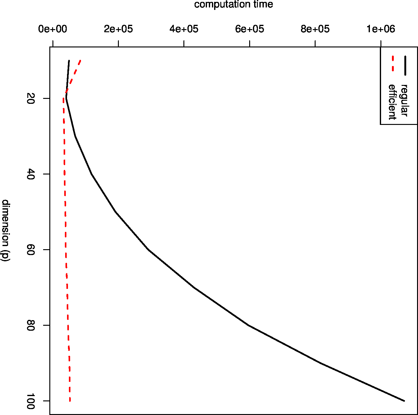
point out that, with the SVD-trick above, the number of computation operations reduces from [math]\mathcal{O}(p^3)[/math] to [math]\mathcal{O}(p n^2)[/math]. In addition, they point out that this computational short-cut can be used in combination with other loss functions, for instance that of standard generalized linear models (see Chapter Ridge logistic regression ). This computation can is illustrated in Figure, which shows the substantial gain in computation time of the evaluation of the ridge regression estimator using the efficient over the naive implementation against the dimension [math]p[/math]. Details of this figure are provided in Question.

Computation time of the evaluation of the ridge regression estimator using the naive and efficient implementation against the dimension [math]p[/math].

The inversion of the [math]p \times p[/math]-dimensional matrix can be avoided in an other way. Hereto one needs the Woodbury identity. Let [math]\mathbf{A}[/math], [math]\mathbf{U}[/math] and [math]\mathbf{V}[/math] be [math]p \times p[/math]-, [math]p \times n[/math]- and [math]n \times p[/math]-dimensional matrices, respectively. The (simplified form of the) Woodbury identity then is:

[[math]] \begin{eqnarray*} (\mathbf{A} + \mathbf{U} \mathbf{V})^{-1} & = & \mathbf{A}^{-1} - \mathbf{A}^{-1} \mathbf{U} (\mathbf{I}_{nn} + \mathbf{V} \mathbf{A}^{-1} \mathbf{U})^{-1} \mathbf{V} \mathbf{A}^{-1}. \end{eqnarray*} [[/math]]

Application of the Woodbury identity to the matrix inverse in the ridge estimator of the regression parameter gives:

[[math]] \begin{eqnarray*} (\lambda \mathbf{I}_{pp} + \mathbf{X}^{\top} \mathbf{X})^{-1} & = & \lambda^{-1} \mathbf{I}_{pp} - \lambda^{-2} \mathbf{X}^{\top} (\mathbf{I}_{nn} + \lambda^{-1} \mathbf{X} \mathbf{X}^{\top})^{-1} \mathbf{X}. \end{eqnarray*} [[/math]]

This gives:

[[math]] \begin{eqnarray} \label{form.effRidgeEstimator} (\lambda \mathbf{I}_{pp} + \mathbf{X}^{\top} \mathbf{X})^{-1} \mathbf{X}^{\top} \mathbf{Y} & = & \lambda^{-1} \mathbf{X}^{\top} \mathbf{Y} - \lambda^{-2} \mathbf{X}^{\top} (\mathbf{I}_{nn} + \lambda^{-1} \mathbf{X} \mathbf{X}^{\top})^{-1} \mathbf{X} \mathbf{X}^{\top} \mathbf{Y} \end{eqnarray} [[/math]]

The inversion of the [math]p \times p[/math]-dimensional matrix [math]\lambda \mathbf{I}_{pp} + \mathbf{X}^{\top} \mathbf{X}[/math] is thus replaced by that of the [math]n \times n[/math]-dimensional matrix [math]\mathbf{I}_{nn} + \lambda^{-1} \mathbf{X} \mathbf{X}^{\top}[/math]. In addition, this expression of the ridge regression estimator avoids the singular value decomposition of [math]\mathbf{X}[/math], which may in some cases introduce additional numerical errors (e.g. at the level of machine precision).

General References

van Wieringen, Wessel N. (2021). "Lecture notes on ridge regression". arXiv:1509.09169 [stat.ME].

References

- Hoerl, A. E. and Kennard, R. W. (1970).Ridge regression: biased estimation for nonorthogonal problems.Technometrics, 12(1), 55--67
- 2.0 2.1 Harville, D. A. (2008).Matrix Algebra From a Statistician's Perspective.Springer, New York
- 3.0 3.1 Fletcher, R. (2008).Practical Methods of Optimization, 2nd Edition.John Wiley, New York
- Horn, R. A. and Johnson, C. R. (2012).Matrix analysis.Cambridge University Press
- Hastie, T. and Tibshirani, R. (2004).Efficient quadratic regularization for expression arrays.Biostatistics, 5(3), 329--340