Ridge logistic regression

[math] \require{textmacros} \def \bbeta {\bf \beta} \def\fat#1{\mbox{\boldmath$#1$}} \def\reminder#1{\marginpar{\rule[0pt]{1mm}{11pt}}\textbf{#1}} \def\SSigma{\bf \Sigma} \def\ttheta{\bf \theta} \def\aalpha{\bf \alpha} \def\bbeta{\bf \beta} \def\ddelta{\bf \delta} \def\eeta{\bf \eta} \def\llambda{\bf \lambda} \def\ggamma{\bf \gamma} \def\nnu{\bf \nu} \def\vvarepsilon{\bf \varepsilon} \def\mmu{\bf \mu} \def\nnu{\bf \nu} \def\ttau{\bf \tau} \def\SSigma{\bf \Sigma} \def\TTheta{\bf \Theta} \def\XXi{\bf \Xi} \def\PPi{\bf \Pi} \def\GGamma{\bf \Gamma} \def\DDelta{\bf \Delta} \def\ssigma{\bf \sigma} \def\UUpsilon{\bf \Upsilon} \def\PPsi{\bf \Psi} \def\PPhi{\bf \Phi} \def\LLambda{\bf \Lambda} \def\OOmega{\bf \Omega} [/math]

Ridge penalized estimation is not limited to the standard linear regression model, but may be used to estimate (virtually) any model. Here we illustrate how it may be used to fit the logistic regression model. To this end we first recap this model and the (unpenalized) maximum likelihood estimation of its parameters. After which the model is estimated by means of ridge penalized maximum likelihood, which will turn out to be a relatively straightforward modification of unpenalized estimation.

Logistic regression

The logistic regression model explains a binary response variable (through some transformation) by a linear combination of a set of covariates (as in the linear regression model). Denote this response of the [math]i[/math]-th sample by [math]Y_i[/math] with [math]Y_i \in \{ 0, 1 \}[/math] for [math]i=1, \ldots, n[/math]. The [math]n[/math]-dimensional column vector [math]\mathbf{Y}[/math] stacks these [math]n[/math] responses. For each sample information on the [math]p[/math] explanatory variables [math]X_{i,1}, \ldots, X_{i,p}[/math] is available. In row vector form this information is denoted [math]\mathbf{X}_{i,\ast} = (X_{i,1}, \ldots, X_{i,p})[/math]. Or, in short, [math]\mathbf{X}_i[/math] when the context tolerates no confusion. The [math](n \times p)[/math]-dimensional matrix [math]\mathbf{X}[/math] aggregates these vectors, such that [math]\mathbf{X}_i[/math] is the [math]i[/math]-th row vector.

The binary response cannot be modelled as in the linear model like [math]Y_i = \mathbf{X}_i \bbeta + \varepsilon_i[/math]. With each element of [math]\mathbf{X}_i[/math] and [math]\bbeta[/math] assuming a value in [math]\mathbb{R}^p[/math], the linear predictor is not restricted to the domain of the response. This is resolved by modeling [math]p_i = P(Y_i = 1)[/math] instead. Still the linear predictor may exceed the domain of the response ([math]p_i \in [0,1][/math]). Hence, a transformation is applied to map [math]p_i[/math] to [math]\mathbb{R}[/math], the range of the linear predictor.

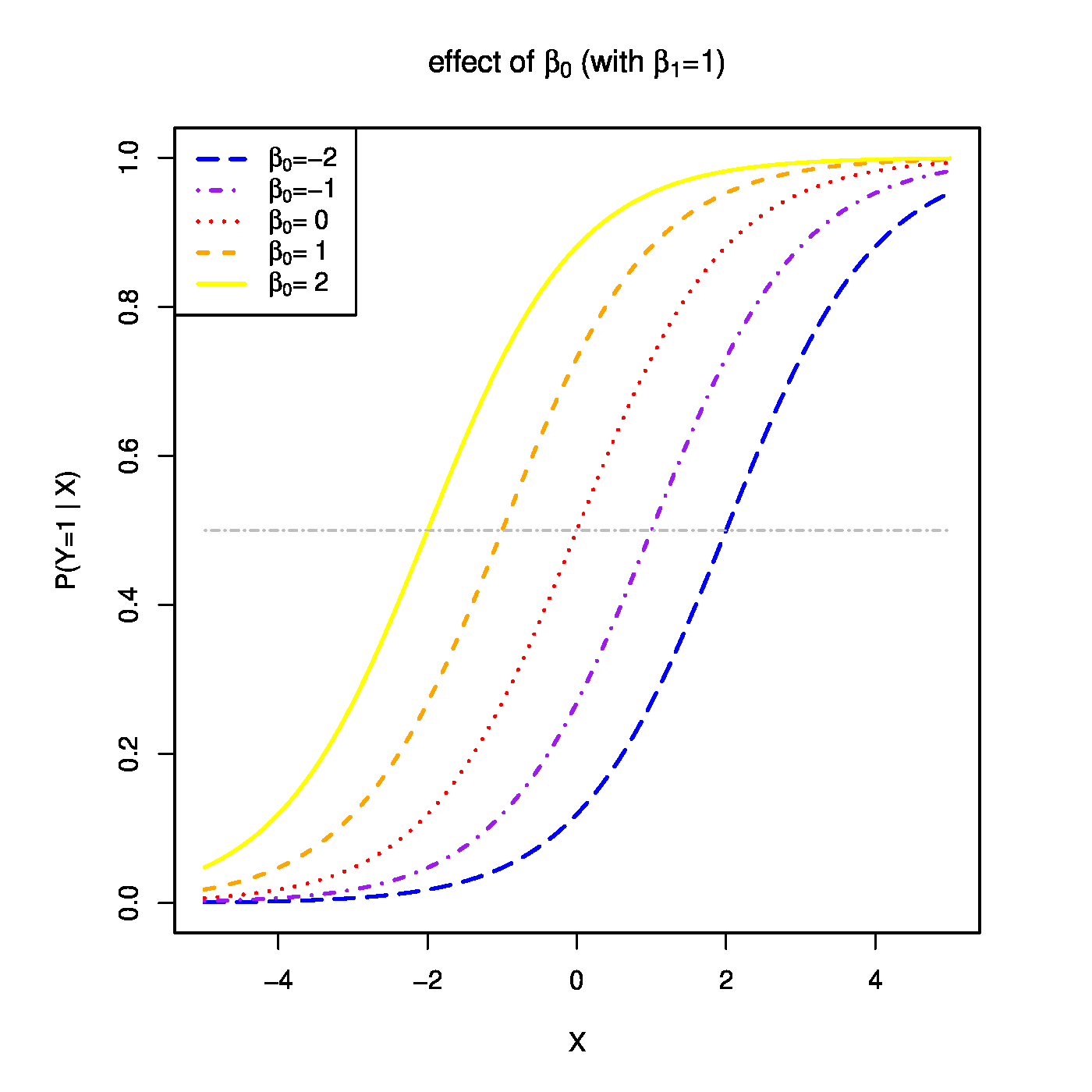
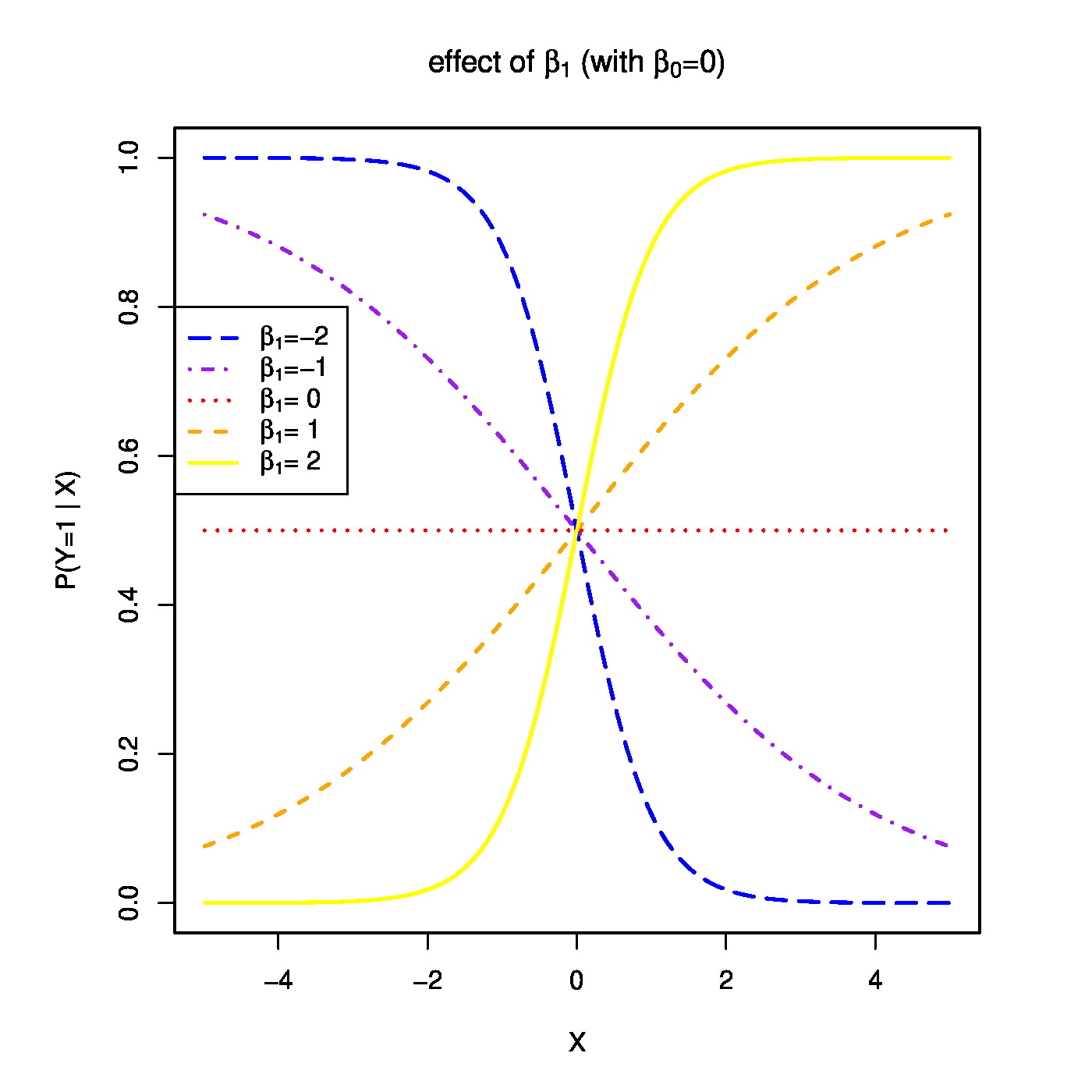
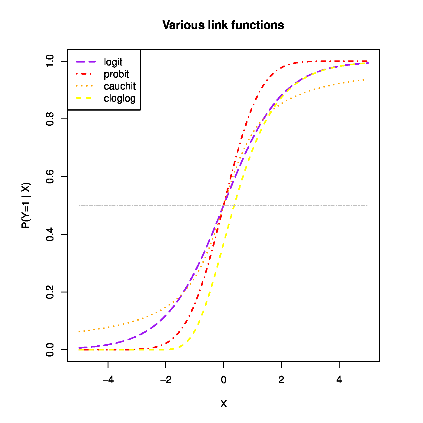
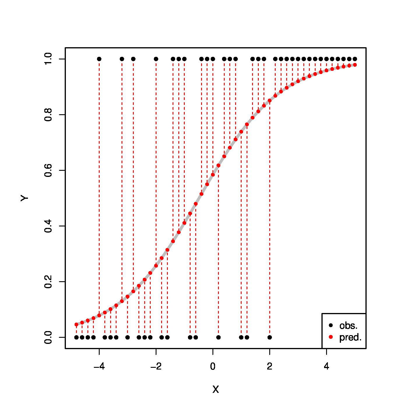
Top row, left panel: the response curve for various choices of the intercept [math]\beta_0[/math]. Top row, right panel: the response curve for various choices of the regression coefficent [math]\beta_1[/math]. Bottom row, left panel: the responce curve for various choices of the link function. Bottom panel, right panel: observations, fits and their deviations.

The transformation associated with the logistic regression model is the logarithm of the odds, with the odds defined as: [math]\mbox{'' odds''} = P(\mbox{succes}) / P(\mbox{failure}) = p_i/ (1-p_i)[/math]. The logistic model is then written as [math]\log[ p_i / (1-p_i)] = \mathbf{X}_i \bbeta[/math] for all [math]i[/math]. Or, expressed in terms of the response:

[[math]] \begin{eqnarray*} p_i & = & P(Y_i = 1) \, \, \, = \, \, \, g^{-1}(\mathbf{X}_i; \bbeta) \, \, \, = \, \, \,\exp(\mathbf{X}_i \bbeta) [1 + \exp(\mathbf{X}_i \bbeta) ]^{-1}. \end{eqnarray*} [[/math]]

The function [math]g(\cdot; \cdot)[/math] is called the link function. It links the response to the explanatory variables. The one above is called the logistic link function. Or short, logit. The regression parameters have tangible interpretations. When the first covariate represents the intercept, i.e. [math]X_{i,j} = 1[/math] for all [math]i[/math], then [math]\beta_1[/math] determines where the link function equals a half when all other covariates fail to contribute to the linear predictor (i.e. where [math]P (Y_i = 1 \, | \, \mathbf{X}_{i}) = 0.5[/math] when [math]\mathbf{X}_{i} \bbeta = \beta_1[/math]). This is illustrated in the top-left panel of Figure for various choices of the intercept. On the other hand, the regression parameters are directly related to the odds ratio: [math]\mbox{'' odds ratio''} = \mbox{odds}(X_{i,j}+1) / \mbox{odds}(X_{i,j}) = \exp(\beta_j)[/math]. Hence, the effect of a unit change in the [math]j[/math]-th covariate on the odds ratio is [math]\exp(\beta_j)[/math] (see Figure, top-right panel). Other link functions (depicted in Figure, bottom-left panel) are common, e.g. the probit: [math]p_i = \Phi_{0,1}(\mathbf{X}_i \bbeta)[/math]; the cloglog: [math]p_i = \frac{1}{\pi} \arctan(\mathbf{X}_i \bbeta) + \frac{1}{2}[/math]; the Cauchit: [math]p_i = \exp[ - \exp(\mathbf{X}_i \bbeta)][/math]. All these link function are invertible. Irrespective of the choice of the link function, the binary data are thus modelled as [math]Y_i \sim \mathcal{B}[g^{-1}(\mathbf{X}_i; \bbeta), 1][/math]. That is, as a single draw from the Binomial distribution with success probability [math]g^{-1}(\mathbf{X}_i; \bbeta)[/math].

Let us now estimate the parameter of the logistic regression model by means of the maximum likelihood method. The likelihood of the experiment is then:

[[math]] \begin{eqnarray*} L(\mathbf{Y} \, | \, \mathbf{X}; \bbeta) & = & \prod_{i=1}^n \big[ P(Y_i = 1 \, | \, \mathbf{X}_i) \big]^{Y_i} \big[ P(Y_i = 0 \, | \, \mathbf{X}_i) \big]^{1-Y_i}. \end{eqnarray*} [[/math]]

After taking the logarithm and some ready algebra, the log-likelihood is found to be:

[[math]] \begin{eqnarray*} \mathcal{L}(\mathbf{Y} \, | \, \mathbf{X}; \bbeta) & = & \sum\nolimits_{i=1}^n \big\{ Y_i \mathbf{X}_i \bbeta - \log [ 1 + \exp(\mathbf{X}_i \bbeta) ] \big\}. \end{eqnarray*} [[/math]]

Differentiate the log-likelihood with respect to [math]\bbeta[/math], equate it zero, and obtain the estimating equation for [math]\bbeta[/math]:

[[math]] \begin{eqnarray} \label{form:logisticRidge_estimatingEquationOfBeta} \frac{\partial \mathcal{L}}{\partial \bbeta } & = & \sum_{i=1}^n \Big[ Y_i - \frac{\exp(\mathbf{X}_i \bbeta)}{ 1 + \exp(\mathbf{X}_i \bbeta)} \Big] \mathbf{X}_i^{\top} \, \, \, = \, \, \, \mathbf{0}_p. \end{eqnarray} [[/math]]

The ML estimate of [math]\bbeta[/math] strikes a (weighted by the [math]\mathbf{X}_i[/math]) balance between observation and model. Put differently (and illustrated in the bottom-right panel of Figure), a curve is fit through data by minimizing the distance between them: at the ML estimate of [math]\bbeta[/math] a weighted average of their deviations is zero.

The maximum likelihood estimate of [math]\bbeta[/math] is evaluated by solving Equation (\ref{form:logisticRidge_estimatingEquationOfBeta}) with respect to [math]\bbeta[/math] by means of the Newton-Raphson algorithm. The Newton-Raphson algorithm iteratively finds the zeros of a smooth enough function [math]f(\cdot)[/math]. Let [math]x_0[/math] denote an initial guess of the zero. Then, approximate [math]f(\cdot)[/math] around [math]x_0[/math] by means of a first order Taylor series: [math]f(x) \approx f(x_0) + (x - x_0) \, (d f / d x) |_{x=x_0}[/math]. Solve this for [math]x[/math] and obtain: [math]x = x_0 - [ (d f / d x) |_{x=x_0} ]^{-1} f(x_0)[/math]. Let [math]x_1[/math] be the solution for [math]x[/math], use this as the new guess and repeat the above until convergence. When the function [math]f(\cdot)[/math] has multiple arguments, is vector-valued and denoted by [math]\vec{\mathbf{f}}[/math], and the Taylor approximation becomes: [math]\vec{\mathbf{f}}(\mathbf{x}) \approx f(\mathbf{x}_0) + J \vec{\mathbf{f}} \big|_{\mathbf{x}=\mathbf{x}_0} (\mathbf{x} - \mathbf{x}_0)[/math] with

[[math]] \begin{eqnarray*} J \vec{\mathbf{f}} = \left( \begin{array}{llll} \frac{\partial f_1}{\partial x_1} & \frac{\partial f_1}{\partial x_2} & \ldots & \frac{\partial f_1}{\partial x_p} \\ \frac{\partial f_1}{\partial x_1} & \frac{\partial f_2}{\partial x_2} & \ldots & \frac{\partial f_2}{\partial x_p} \\ \vdots & \vdots & \ddots & \vdots \\ \frac{\partial f_q}{\partial x_1} & \frac{\partial f_q}{\partial x_2} & \ldots & \frac{\partial f_q}{\partial x_p} \end{array} \right), \end{eqnarray*} [[/math]]

the Jacobi matrix. An update of [math]x_0[/math] is now readily constructed by solving (the approximation for) [math]\vec{\mathbf{f}}(\mathbf{x}) = \mathbf{0}[/math] for [math]\mathbf{x}[/math].

When applied here to the maximum likelihood estimation of the regression parameter [math]\bbeta[/math] of the logistic regression model, the Newton-Raphson update is:

[[math]] \begin{eqnarray*} \hat{\bbeta}^{\mbox{{\scriptsize new}}} & = & \hat{\bbeta}^{\mbox{{\scriptsize old}}} - \Big( \frac{\partial^2 \mathcal{L}}{\partial \bbeta \partial \bbeta^{\top}} \Big)^{-1} \Big|_{\bbeta = \hat{\bbeta}^{\mbox{{\tiny old}}} } \, \, \frac{\partial \mathcal{L}}{\partial \bbeta } \Big|_{\bbeta = \hat{\bbeta}^{\mbox{{\tiny old}}} } \end{eqnarray*} [[/math]]

where the Hessian of the log-likelihood equals:

[[math]] \begin{eqnarray*} \frac{\partial^2 \mathcal{L}}{\partial \bbeta \partial \bbeta^{\top}} & = & - \sum\nolimits_{i=1}^n \frac{\exp(\mathbf{X}_i \bbeta)}{ [1 + \exp(\mathbf{X}_i \bbeta)]^2} \mathbf{X}_i^{\top} \mathbf{X}_i. \end{eqnarray*} [[/math]]

Iterative application of this updating formula converges to the ML estimate of [math]\bbeta[/math].

The Newton-Raphson algorithm is often reformulated as an iteratively re-weighted least squares (IRLS) algorithm. Hereto, first write the gradient and Hessian in matrix notation:

[[math]] \begin{eqnarray*} \frac{\partial \mathcal{L}}{\partial \bbeta } \, \, \, = \, \, \, \mathbf{X}^{\top} [\mathbf{Y} - \vec{\mathbf{g}}^{-1}( \mathbf{X}; \bbeta)] & \mbox{ and } & \frac{\partial^2 \mathcal{L}}{\partial \bbeta \partial \bbeta^{\top}} \, \, \, = \, \, \, - \mathbf{X}^{\top} \mathbf{W} \mathbf{X}, \end{eqnarray*} [[/math]]

where [math]\vec{\mathbf{g}}^{-1}( \mathbf{X}; \bbeta) = [g^{-1}( \mathbf{X}_{1, \ast}; \bbeta), \ldots, g^{-1}( \mathbf{X}_{n, \ast}; \bbeta)]^{\top}[/math] with [math]g^{-1}(\cdot; \cdot) = \exp(\cdot; \cdot) / [1 + \exp(\cdot; \cdot)][/math] and [math]\mathbf{W}[/math] diagonal with [math](\mathbf{W})_{ii} = \exp(\mathbf{X}_i \hat{\bbeta}^{\mbox{{\scriptsize old}}} ) [ 1 + \exp(\mathbf{X}_i \hat{\bbeta}^{\mbox{{\scriptsize old}}} ) ]^{-2}[/math]. The notation [math]\mathbf{W}[/math] was already used in Chapter Generalizing ridge regression and, generally, refers to a (diagonal) weight matrix with the choice of the weights depending on the context. The updating formula of the estimate then becomes:

[[math]] \begin{eqnarray*} \hat{\bbeta}^{\mbox{{\scriptsize new}}} & = & \hat{\bbeta}^{\mbox{{\scriptsize old}}} + (\mathbf{X}^{\top} \mathbf{W} \mathbf{X})^{-1} \mathbf{X}^{\top} [\mathbf{Y} - \vec{\mathbf{g}}^{-1}( \mathbf{X}; \bbeta^{\mbox{{\scriptsize old}}})] \\ & = & (\mathbf{X}^{\top} \mathbf{W} \mathbf{X})^{-1} \mathbf{X}^{\top} \mathbf{W} \{ \mathbf{X} \hat{\bbeta}^{\mbox{{\scriptsize old}}} + \mathbf{W}^{-1} [\mathbf{Y} - \vec{\mathbf{g}}^{-1}( \mathbf{X}; \bbeta^{\mbox{{\scriptsize old}}})] \} \\ & = & (\mathbf{X}^{\top} \mathbf{W} \mathbf{X})^{-1} \mathbf{X}^{\top} \mathbf{W} \mathbf{Z}, \end{eqnarray*} [[/math]]

where [math]\mathbf{Z} = \{ \mathbf{X} \hat{\bbeta}^{\mbox{{\scriptsize old}}} + \mathbf{W}^{-1} [\mathbf{Y} - \vec{\mathbf{g}}^{-1}( \mathbf{X}; \bbeta^{\mbox{{\scriptsize old}}})] \}[/math]. The Newton-Raphson update is thus the solution to the following weighted least squares problem:

[[math]] \begin{eqnarray*} \hat{\bbeta}^{\mbox{{\scriptsize new}}} & = & \arg \min_{\bbeta} ~ (\mathbf{Z} - \mathbf{X} \bbeta)^{\top} \mathbf{W} (\mathbf{Z} - \mathbf{X} \bbeta). \end{eqnarray*} [[/math]]

Effectively, at each iteration the adjusted response [math]\mathbf{Z}[/math] is regressed on the covariates that comprise [math]\mathbf{X}[/math]. For more on logistic regression confer the monograph of .

Ridge estimation

High-dimensionally, the linear predictor [math]\mathbf{X} \bbeta[/math] may be uniquely defined, but the maximum likelihood estimator of the logistic regression parameter is not. Assume [math]p \gt n[/math] and an estimate [math]\hat{\bbeta}[/math] available. Due to the high-dimensionality, the null space of [math]\mathbf{X}[/math] is non-trivial. Hence, let [math]\ggamma \in \mbox{null}(\mbox{span}(\mathbf{X}))[/math]. Then: [math]\mathbf{X} \hat{\bbeta} = \mathbf{X} \hat{\bbeta} + \mathbf{X} \ggamma = \mathbf{X} (\hat{\bbeta} + \ggamma)[/math]. As the null space is a [math]p-n[/math]-dimensional subspace, [math]\ggamma[/math] need not equal zero. Hence, an infinite number of estimators of the logistic regression parameter exists that yield the same loglikelihood. Augmentation of the loss function with a ridge penalty resolves the matter, as their sum is strictly concave in [math]\bbeta[/math] (not convex as a maximizer rather than a minimizer is sought here) and thereby has a unique maximum.

The binary nature of the response may bring about another problem, called separable data, that frustates the estimation of the logistic regression estimator. High-dimensionally, this problem is virtually always encountered. Separable data refer to the situation where the covariate space can be separated by a hyperplane such that the samples with indices in the set [math]\{i : Y_i =0\}[/math] fall on one side of this hyperplane while those with an index in the set [math]\{i : Y_i =1\}[/math] on the other. High-dimensionally, such a hyperplane can always be found (unless there is at least one pair of samples with a common variate vector, i.e. [math]\mathbf{X}_{i,\ast} = \mathbf{X}_{i',\ast}[/math], with different responses [math]Y_i \not= Y_{i'}[/math]). The existence of a separating hyperplane implies that the optimal fit is perfect and all samples have -- according to the fitted logistic regression model -- a probability of one of being assigned to the correct outcome, i.e. [math]P(Y_i = 1 \, | \, \mathbf{X}_i)[/math] equals either zero or one. Consequently, the loglikelihood vanishes, cf.:

[[math]] \begin{eqnarray*} \mathcal{L}(\mathbf{Y} \, | \, \mathbf{X}; \bbeta) & = & \sum\nolimits_{i=1}^n Y_i \log [ P(Y_i = 1 \, | \, \mathbf{X}_i)] + (1-Y_i) \log [ P(Y_i = 0 \, | \, \mathbf{X}_i) \big] \, \, \, = \, \, \, 0, \end{eqnarray*} [[/math]]

and does no longer involve the logistic regression parameter. The logistic regression parameter is then to be chosen such that [math]P(Y_i = 1 \, | \, \mathbf{X}_i) = \exp(\mathbf{X}_i \bbeta) [1 + \exp(\mathbf{X}_i \bbeta)]^{-1} \in \{ 0, 1\}[/math] (depending on whether [math]Y_i[/math] is indeed of the ‘1’ class). This only occurs when (some) elements of [math]\bbeta[/math] equal (minus) infinity. Hence, the logistic regression parameter cannot be learned from separable data (which high-dimensional data generally are).

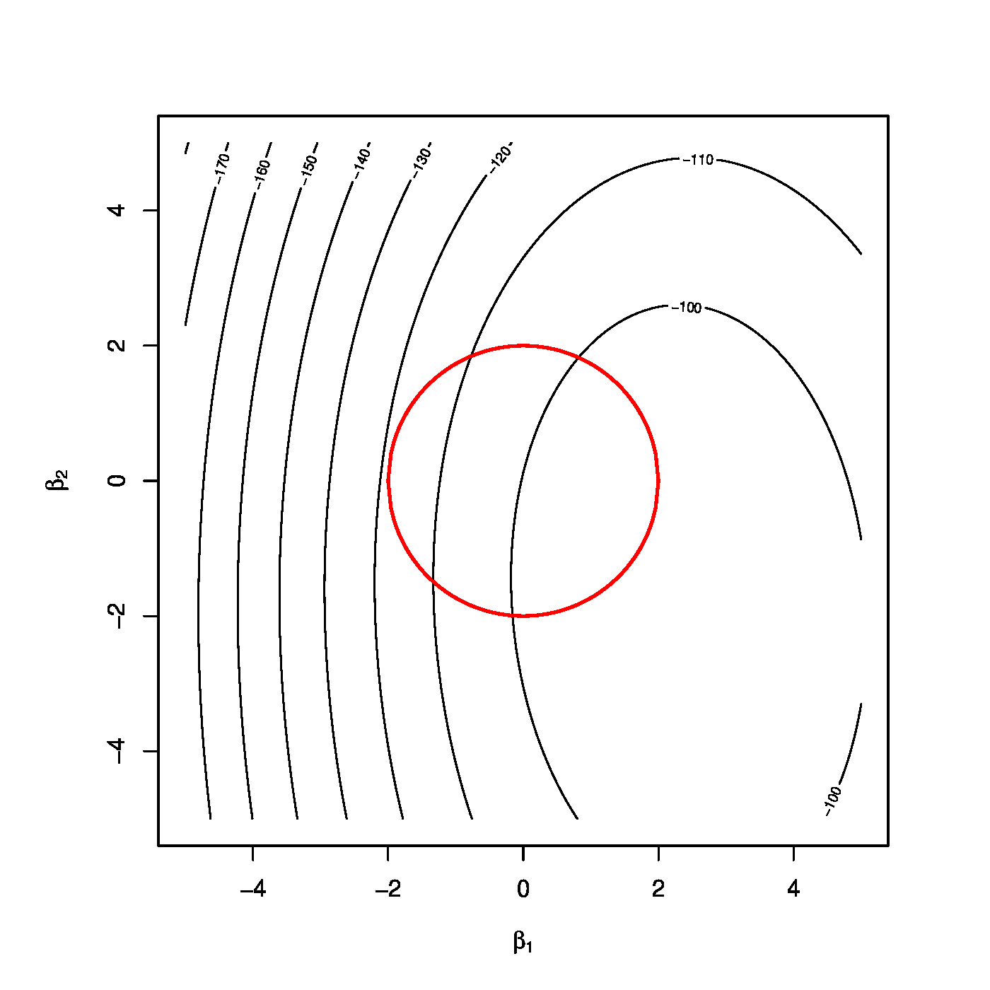
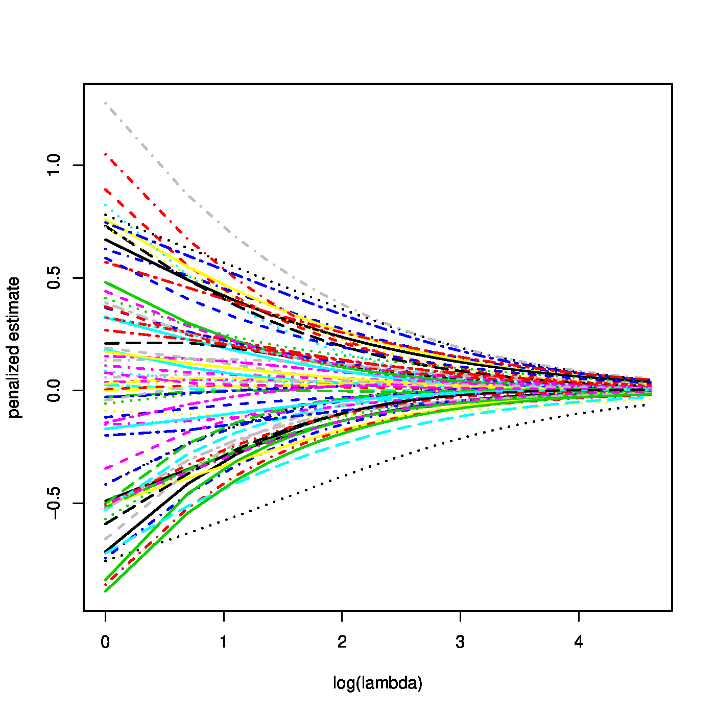
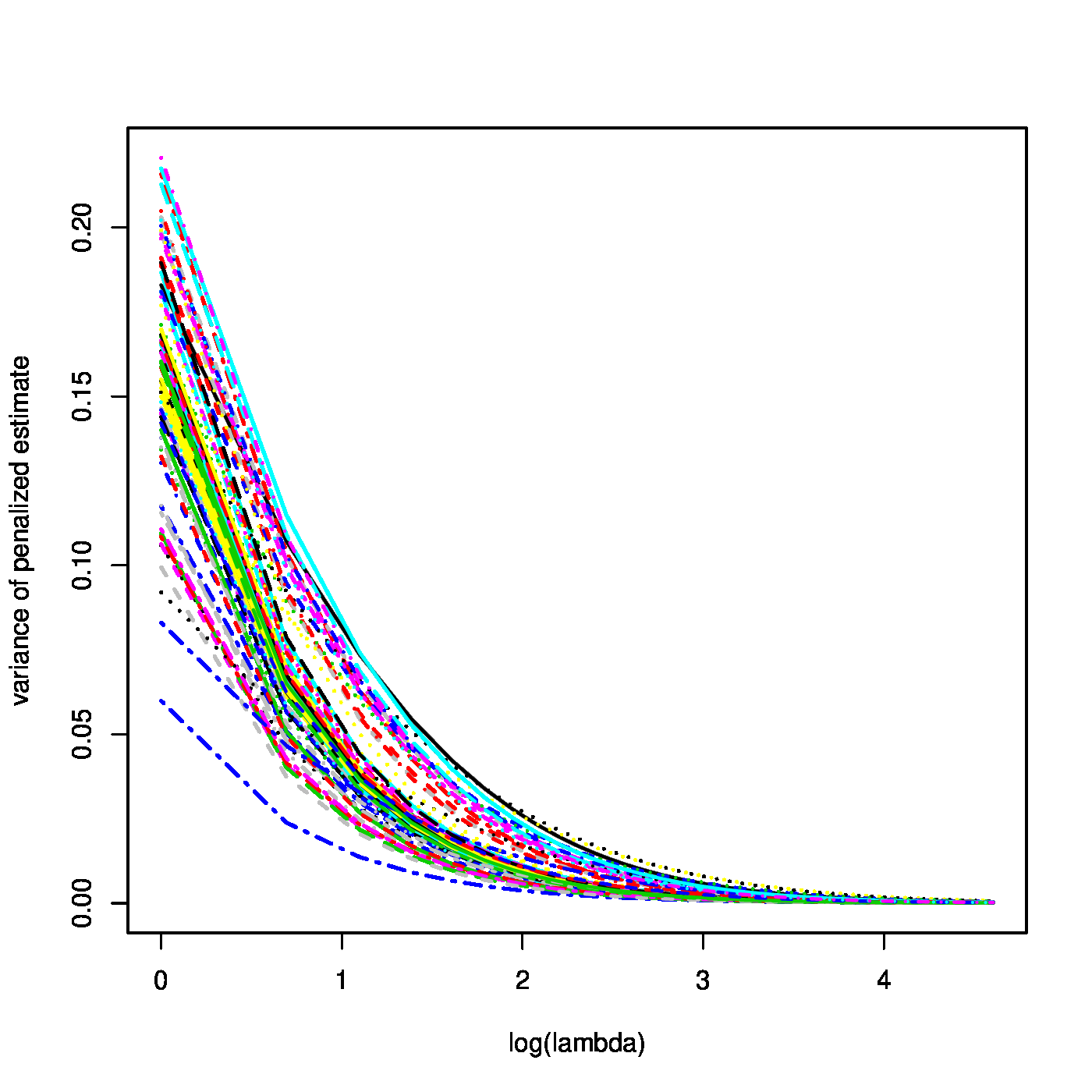
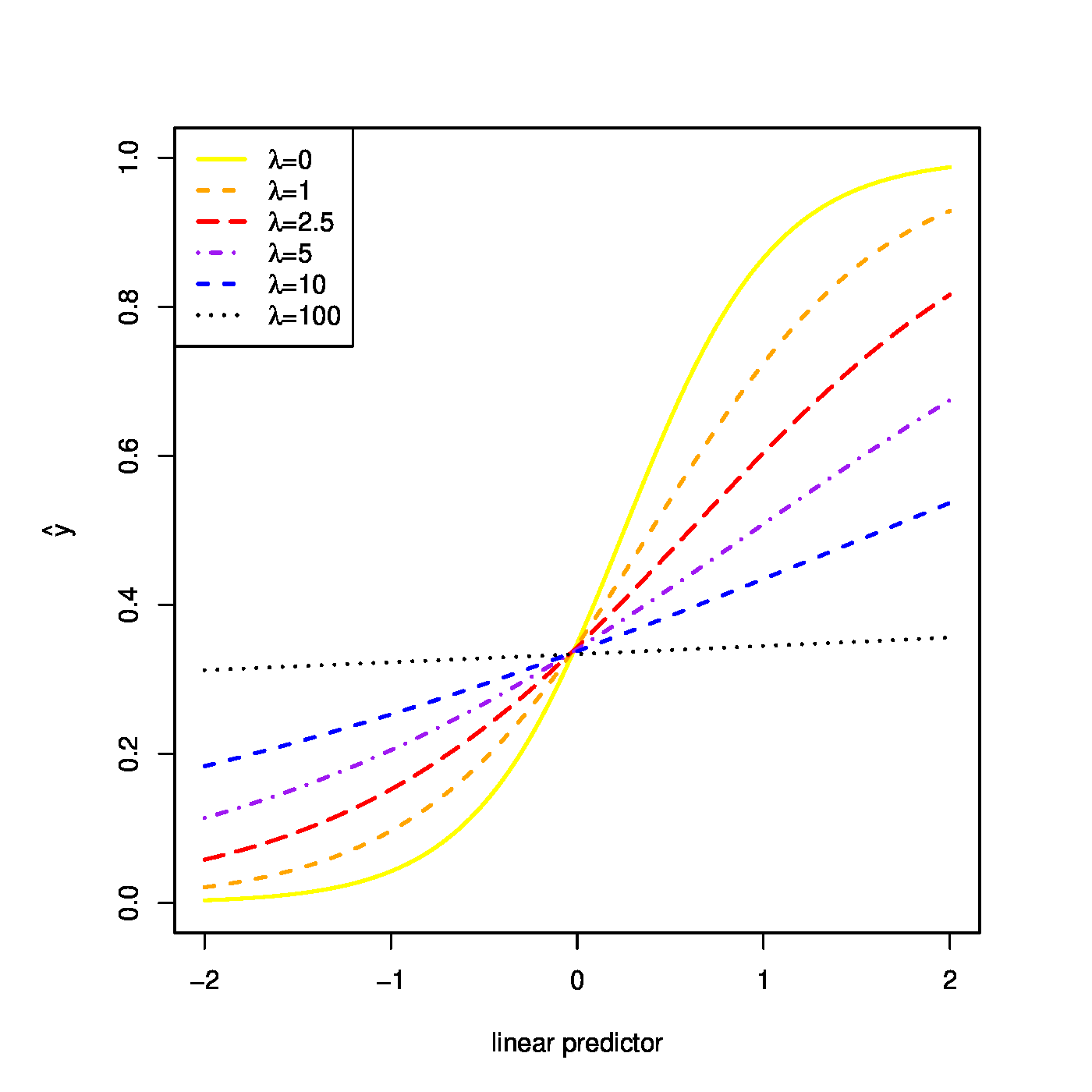
Top row, left panel: contour plot of the penalized log-likelihood of a logistic regression model with the ridge constraint (red line). Top row, right panel: the regularization paths of the ridge estimator of the logistic regression parameter. Bottom row, left panel: variance of the ridge estimator of the logistic regression parameter against the logarithm of the penalty parameter. Bottom panel, right panel: the predicted success probability versus the linear predictor for various choices of the penalty parameter.

Ridge maximum likelihood estimates of the logistic model parameters are found by the maximization of the ridge penalized loglikelihood (cf. ):

[[math]] \begin{eqnarray*} \mathcal{L}^{\mbox{{\tiny pen}}}(\mathbf{Y}, \mathbf{X}; \bbeta, \lambda) & = & \mathcal{L} (\mathbf{Y}, \mathbf{X}; \bbeta) - \tfrac{1}{2} \lambda \| \bbeta \|_2^2 \\ & = & \sum\nolimits_{i=1}^n \big\{ Y_i \mathbf{X}_i \bbeta - \log [ 1 + \exp(\mathbf{X}_i \bbeta) ] \big\} - \tfrac{1}{2} \lambda \bbeta^{\top} \bbeta, \end{eqnarray*} [[/math]]

where the second summand is the ridge penalty (the sum of the square of the elements of [math]\bbeta[/math]) with [math]\lambda[/math] the penalty parameter. Penalization of the loglikelihood now amounts to the substraction of the ridge penalty. This is due to the fact that the estimator is now defined as the maximizer (instead of a minimizer) of the loss function. Moreover, the [math]\tfrac{1}{2}[/math] in front of the penalty is only there to simply derivations later, and could in principle be absorped in the penalty parameter. Finally, the augmentation of the loglikelihood with the ridge penalty ensures the existence of a unique estimator. The loglikelihood need not be strictly concave, but the ridge penalty, [math]-\tfrac{1}{2} \| \bbeta \|_2^2[/math], is. Together they form the ridge penalized loglikelihood above, which is thus also strictly concave. This warrants the existence of a unique maximizer, and a well-defined ridge logistic regression estimator.

The optimization of the ridge penalized loglikelihood associated with the logistic regression model proceeds, due to the differentiability of the penalty, fully analogous to the unpenalized case and uses the Newton-Raphson algorithm for solving the (penalized) estimating equation. Hence, the unpenalized ML estimation procedure is modified straightforwardly by replacing gradient and Hessian by their ‘penalized’ counterparts:

[[math]] \begin{eqnarray*} \frac{\partial \mathcal{L}^{\mbox{{\tiny pen}}}}{\partial \bbeta } \, \, \, = \, \, \, \frac{\partial \mathcal{L}}{\partial \bbeta } - \lambda \bbeta & \mbox{ and } & \frac{\partial^2 \mathcal{L}^{\mbox{{\tiny pen}}}}{\partial \bbeta \partial \bbeta^{\top}} \, \, \, = \, \, \, \frac{\partial^2 \mathcal{L}}{\partial \bbeta \partial \bbeta^{\top}} - \lambda \mathbf{I}_{pp}. \end{eqnarray*} [[/math]]

With these at hand, the Newton-Raphson algorithm is (again) reformulated as an iteratively re-weighted least squares algorithm with the updating step changing accordingly to:

[[math]] \begin{eqnarray*} \hat{\bbeta}^{\mbox{{\scriptsize new}}} (\lambda) & = & \hat{\bbeta}^{\mbox{{\scriptsize old}}}(\lambda) + \mathbf{V}^{-1} \{ \mathbf{X}^{\top} \{ \mathbf{Y} - \vec{\mathbf{g}}^{-1}[ \mathbf{X}; \bbeta^{\mbox{{\scriptsize old}}} (\lambda) ] \} - \lambda \bbeta^{\mbox{{\scriptsize old}}} )\lambda) \} \\ & = & \mathbf{V}^{-1} \mathbf{V} \hat{\bbeta}^{\mbox{{\scriptsize old}}} - \lambda \mathbf{V}^{-1} \hat{\bbeta}^{\mbox{{\scriptsize old}}} (\lambda) + \mathbf{V}^{-1} \mathbf{X}^{\top} \mathbf{W} \mathbf{W}^{-1} \{\mathbf{Y} - \vec{\mathbf{g}}^{-1}[ \mathbf{X}; \bbeta^{\mbox{{\scriptsize old}}}(\lambda)]\} \\ & = & \mathbf{V}^{-1} \mathbf{X}^{\top} \mathbf{W} \big( \mathbf{X} \hat{\bbeta}^{\mbox{{\scriptsize old}}} (\lambda) + \mathbf{W}^{-1} \{ \mathbf{Y} - \vec{\mathbf{g}}^{-1}[ \mathbf{X}; \bbeta^{\mbox{{\scriptsize old}}}(\lambda)] \} \big) \\ & = & (\mathbf{X}^{\top} \mathbf{W} \mathbf{X} + \lambda \mathbf{I}_{pp} )^{-1} \mathbf{X}^{\top} \mathbf{W} \mathbf{Z}, \end{eqnarray*} [[/math]]

where [math]\mathbf{V} = \mathbf{X}^{\top} \mathbf{W} \mathbf{X} + \lambda \mathbf{I}_{pp}[/math] and [math]\mathbf{W}[/math] and [math]\mathbf{Z}[/math] as before. Hence, use this to update the estimate of [math]\bbeta[/math] until convergence, which yields the desired ridge ML estimate.

Obviously, the ridge estimate of the logistic regression parameter tends to zero as [math]\lambda \rightarrow \infty[/math]. Now consider a linear predictor with an intercept that is left unpenalized. When [math]\lambda[/math] tends to infinity, all regression coefficients but the intercept vanish. The intercept is left to model the success probability. Hence, in this case [math]\lim_{\lambda \rightarrow \infty} \hat{\beta}_0 (\lambda) = \log [ \tfrac{1}{n} \sum_{i=1}^n Y_i / \tfrac{1}{n} \sum_{i=1}^n (1-Y_i)][/math].

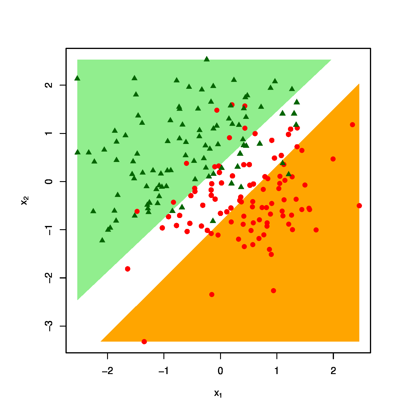
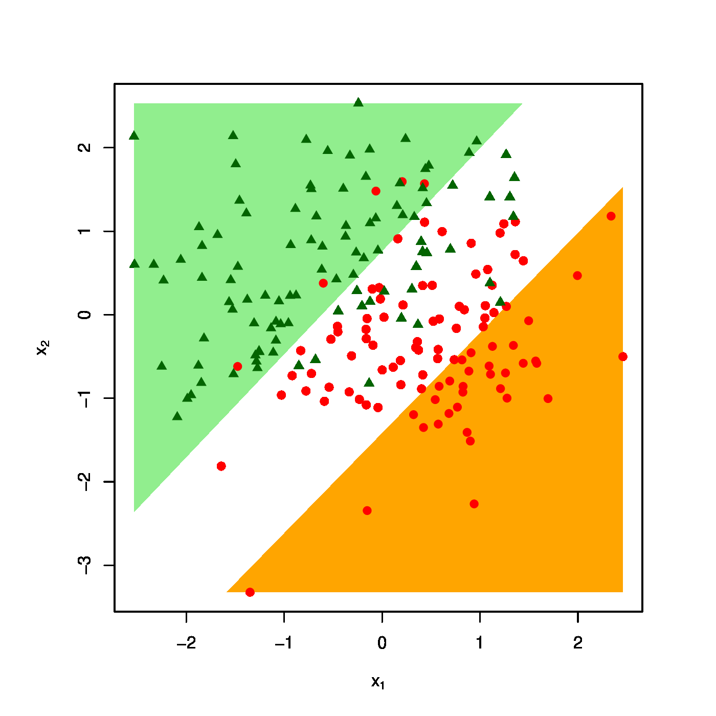
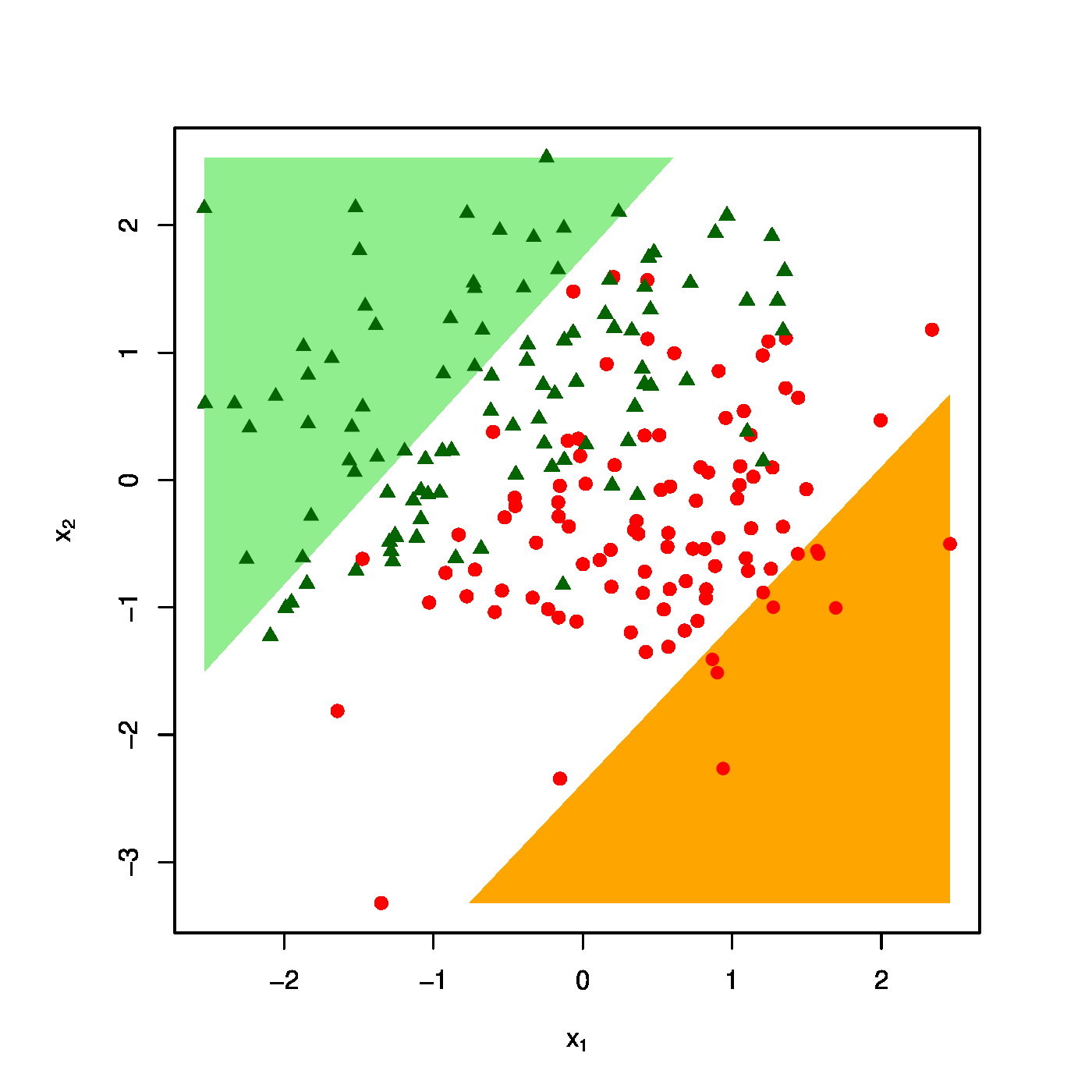
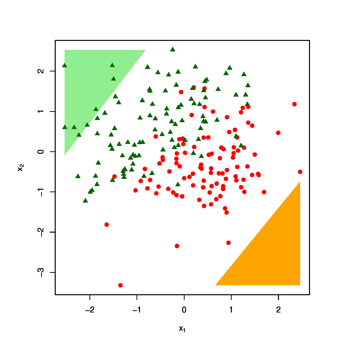
The realized design as scatter plot ([math]X_1[/math] vs [math]X_2[/math] overlayed by the success ([math]\textcolor{red}{RED}[/math]) and failure regions ([math]\textcolor{green}{GREEN}[/math]) for various choices of the penalty parameter: [math]\lambda = 0[/math] (top row, left panel), [math]\lambda = 10[/math] (top row, right panel) [math]\lambda = 40[/math] (bottom row, left panel), [math]\lambda = 100[/math] (bottom row, right panel).

The effect of the ridge penalty on parameter estimates propagates to the predictor [math]\hat{p}_i[/math]. The linear predictor of the linear regression model involving the ridge estimator [math]\mathbf{X}_i \hat{\bbeta}(\lambda)[/math] shrinks towards a common value for each [math]i[/math], leading to a scale difference between observation and predictor (as seen before in Section Illustration ). This behaviour transfers to the ridge logistic regression predictor, as is illustrated on simulated data. The dimension and sample size of these data are [math]p=2[/math] and [math]n=200[/math], respectively. The covariate data are drawn from the standard normal, while that of the response is sampled from a Bernoulli distribution with success probability [math]P(Y_i=1) = \exp(2 X_{i,1} - 2 X_{i,2}) / [ 1 + \exp(2 X_{i,1} - 2 X_{i,2})][/math]. The logistic regression model is estimated from these data by means of ridge penalized likelihood maximization with various choices of the penalty parameter. The bottom right plot in Figure shows the predicted success probability versus the linear predictor for various choices of the penalty parameter. Larger values of the penalty parameter [math]\lambda[/math] flatten the slope of this curve. Consequently, for larger [math]\lambda[/math] more excessive values of the covariates are needed to achieve the same predicted success probability as those obtained with smaller [math]\lambda[/math] at more moderate covariate values. The implications for the resulting classification may become clearer when studying the effect of the penalty parameter on the ‘failure’ and ‘success regions’ respectively defined by:

[math]\{(x_1, x_2) : P({\color{green}{\mathbf{Y=0}}} \, | \, X_1=x_1, X_2=x_2, \hat{\bbeta}(\lambda)) \gt 0.75 \}[/math],

[math]\{(x_1, x_2) : P({\color{red}{\mathbf{Y=1}}} \, | \, X_1=x_1, X_2=x_2, \hat{\bbeta}(\lambda)) \gt 0.75 \}[/math].

This separates the design space in a light red (‘failure’) and light green (‘success’) domain. The white bar between them is the domain where samples cannot be classified with high enough certainty. As [math]\lambda[/math] grows, so does the white area that separates the failure and success regions. Hence, as stronger penalization shrinks the logistic regression parameter estimate towards zero, it produces a predictor that is less outspoken in its class assignments.

Moments

The [math]1^{\mbox{{\tiny st}}}[/math] and [math]2^{\mbox{{\tiny nd}}}[/math] order moment of the ridge ML parameter of the logistic model may be approximated by the final update of the Newton-Raphson estimate. Assume the one-to-last update [math]\hat{\bbeta}^{\mbox{{\scriptsize old}}}[/math] to be non-random and proceed as before with the regular ridge regression estimator of the linear regression model parameter to arrive at:

[[math]] \begin{eqnarray*} \mathbb{E} \big( \hat{\bbeta}^{\mbox{{\scriptsize new}}} \big) & = & (\mathbf{X}^{\top} \mathbf{W} \mathbf{X} + \lambda \mathbf{I}_{pp} )^{-1} \mathbf{X}^{\top} \mathbf{W} \mathbb{E}( \mathbf{Z}), \\ \mbox{Var} \big( \hat{\bbeta}^{\mbox{{\scriptsize new}}} \big) & = & (\mathbf{X}^{\top} \mathbf{W} \mathbf{X} + \lambda \mathbf{I}_{pp} )^{-1} \mathbf{X}^{\top} \mathbf{W} \big[ \mbox{Var} ( \mathbf{Z} ) \big] \mathbf{W} \mathbf{X} ( \mathbf{X}^{\top} \mathbf{W} \mathbf{X} + \lambda \mathbf{I}_{pp} )^{-1}, \end{eqnarray*} [[/math]]

with

[[math]] \begin{eqnarray*} \mathbb{E}(\mathbf{Z}) & = & \{ \mathbf{X} \hat{\bbeta}^{\mbox{{\scriptsize old}}} + \mathbf{W}^{-1} [\mathbb{E}(\mathbf{Y}) - \vec{\mathbf{g}}^{-1}( \mathbf{X}; \bbeta^{\mbox{{\scriptsize old}}})] \}, \\ \mbox{Var}(\mathbf{Z}) & = & \mathbf{W}^{-1} \mbox{Var}(\mathbf{Y}) \mathbf{W}^{-1} = \mathbf{W}^{-1}, \end{eqnarray*} [[/math]]

where the identity [math]\mbox{Var}(\mathbf{Y}) = \mathbf{W}[/math] follows from the variance of a Binomial distributed random variable. From these expressions similar properties as for the ridge ML estimator of the regression parameter of the linear model may be deduced. For instance, the ridge ML estimator of the logistic regression parameter converges to zero as the penalty parameter tends to infinity (confer the top right panel of Figure). Similarly, their variances vanish as [math]\lambda \rightarrow \infty[/math] (illustrated in the bottom left panel of Figure).

For large enough samples sizes, the full distribution of the ridge logistic regression estimator can seen to behave as a normal one. This follows from an approximation of the estimator, which maximizes an approximation of the penalized loglikelihood. The latter exploits the following second order Taylor approximation of [math]\log[ 1+ \exp( \mathbf{X} \bbeta) ][/math] in [math]\bbeta[/math] around [math]\bbeta_0[/math]:

[[math]] \begin{eqnarray*} \log[ 1+ \exp( \mathbf{X} \bbeta) ] & \approx & \log[ 1+ \exp( \mathbf{X} \bbeta_0) ] + [ \vec{\mathbf{g}} (\mathbf{X}; \bbeta_0 )]^{\top} \mathbf{X} ( \bbeta - \bbeta_0) + \tfrac{1}{2} ( \bbeta - \bbeta_0)^{\top} \mathbf{X}^{\top} \mathbf{W}_{0} \mathbf{X} ( \bbeta - \bbeta_0), \end{eqnarray*} [[/math]]

where [math]\mathbf{W}_{0}[/math] is as [math]\mathbf{W}[/math] but with [math]\bbeta_0[/math] substitutes for [math]\hat{\bbeta}^{\mbox{{\tiny old}}}(\lambda)[/math]. Substitute this Taylor approximation in the penalized loglikelihood to obtain an approximation of the latter:

[[math]] \begin{eqnarray*} \mathbf{Y}^{\top} \mathbf{X} \bbeta - \log[ 1+ \exp( \mathbf{X} \bbeta_0) ] - [ \vec{\mathbf{g}} (\mathbf{X}; \bbeta_0 )]^{\top} \mathbf{X} ( \bbeta - \bbeta_0) - \tfrac{1}{2} ( \bbeta - \bbeta_0)^{\top} \mathbf{X}^{\top} \mathbf{W}_{{\beta_0}} \mathbf{X} ( \bbeta - \bbeta_0) - \tfrac{1}{2} \lambda \bbeta^\top \bbeta. \end{eqnarray*} [[/math]]

The desired approximation of the ridge logistic regression estimator is the maximizer of this approximated penalized loglikelihood. Its estimating equation is obtained by equating the derivative of the approximated penalized loglikelihood with respect to [math]\bbeta[/math] to zero:

[[math]] \begin{eqnarray*} \mathbf{X}^{\top} [ \mathbf{Y} - \vec{\mathbf{g}} (\mathbf{X}; \bbeta_0 )] - \mathbf{X}^{\top} \mathbf{W}_{0} \mathbf{X} ( \bbeta - \bbeta_0) - \lambda \bbeta & = & \mathbf{0}_p. \end{eqnarray*} [[/math]]

Solve this estimating equation to find the approximated ridge logistic regression estimator:

[[math]] \begin{eqnarray*} \hat{\bbeta} ( \lambda) & \approx & (\mathbf{X}^{\top} \mathbf{W}_0 \mathbf{X} + \lambda \mathbf{I}_{pp} )^{-1} \{ \mathbf{X}^{\top} [ \mathbf{Y} - \vec{\mathbf{g}} (\mathbf{X}; \bbeta_0 )] + \mathbf{X}^{\top} \mathbf{W}_0 \mathbf{X} \bbeta_0 \} \\ & = & \bbeta_0 + (\mathbf{X}^{\top} \mathbf{W}_0 \mathbf{X} + \lambda \mathbf{I}_{pp} )^{-1} [ \mathbf{U}(\bbeta_0 ) - \lambda \bbeta_0], \end{eqnarray*} [[/math]]

where [math]\mathbf{U} ( \bbeta_0) \mathbf{X}^{\top} [ \mathbf{Y} - \vec{\mathbf{g}} (\mathbf{X}; \bbeta_0 )][/math]. From the expression of the approximated ridge logistic regression estimator, it is immediate that the first two moments are of similar form as those derived above. To obtain the (asymptotic) distribution of the estimator, recognize in [math]\mathbf{U} ( \bbeta_0)[/math] the score function -- the gradient of the loglikelihood -- evaluated at [math]\bbeta_0[/math]. For large sample sizes, the score function with [math]\bbeta_0 = \bbeta[/math] is normally distributed. In particular, [math]\mathbf{U} ( \bbeta) \sim \mathcal{N}(\mathbf{0}_p, \mathbf{X}^{\top} \mathbf{W}_{\beta} \mathbf{X})[/math] for large enough [math]n[/math], where the subscript of [math]\mathbf{W}_{\beta}[/math] is only a reminder that the weights are now evaluated at the true parameter value. Then, for large [math]n[/math]:

[[math]] \begin{eqnarray*} \hat{\bbeta} ( \lambda) & \sim & \mathcal{N} [ \bbeta - \lambda (\mathbf{X}^{\top} \mathbf{W}_\beta \mathbf{X} + \lambda \mathbf{I}_{pp} )^{-1} \bbeta, (\mathbf{X}^{\top} \mathbf{W}_\beta \mathbf{X} + \lambda \mathbf{I}_{pp} )^{-1} - (\mathbf{X}^{\top} \mathbf{W}_\beta \mathbf{X} + \lambda \mathbf{I}_{pp} )^{-2} ], \end{eqnarray*} [[/math]]

in which [math]\lambda[/math] is assumed to be nonrandom. In practice, [math]\bbeta[/math] is of course unknown, but can be estimated, e.g. by the maximum likelihood estimator, which is asymptotically unbiased. % Then, for the above result on the distribution of the ridge logistic regression estimator to have any practical value, we would first have the estimate [math]\bbeta[/math] in an unpenalized fashion -- which requires a large sample size -- and plug this estimate into [math]\mathbf{W}_\beta[/math]. But perhaps the practical value of this asymptotic distribution is in its corroboration of the form of the approximation of the first two moments of the ridge logistic regression estimator.

Constrained estimation

The maximization of the penalized loglikelihood of the logistic regression model can be reformulated as a constrained estimation problem, as was done in Section Constrained estimation for the linear regression model. The ridge logistic regression estimator is thus defined equivalently as:

[[math]] \begin{eqnarray*} \hat{\bbeta}(\lambda) & = & \arg \max\nolimits_{\{\bbeta \in \mathbb{R}^p \, : \, \| \bbeta \|_2^2 \leq c(\lambda) \} } \, \mathcal{L} ( \mathbf{Y}, \mathbf{X}; \bbeta). \end{eqnarray*} [[/math]]

This is illustrated by the top left panel of Figure for the ‘[math]p=2[/math]’-case. It depicts the contours (black lines) of the loglikelihood and the spherical domain of the parameter constraint [math]\{ \bbeta \in \mathbb{R}^2 \, : \, \beta_1^2 + \beta_2^2 \leq c(\lambda) \}[/math] (red line). The parameter constraint can again be interpreted as a means to harness against overfitting, as it prevents the ridge logistic regression estimator from assuming very large values, thereby avoiding a perfect description of the data.

The size of the parameter constraint is -- by identical argumentation as provided in Section Constrained estimation -- equal to [math]c(\lambda) = \| \hat{\bbeta} (\lambda) \|_2^2[/math]. While no explicit expression exists for this size (as none exists for the estimator), it can be bounded. Hereto note that, the ridge logistic regression estimator satisfies: [math]\hat{\bbeta}(\lambda) = \lambda^{-1} \mathbf{X}^{\top} \{ \mathbf{Y} - \vec{\mathbf{g}}^{-1} [\mathbf{X}; \hat{\bbeta}(\lambda)]\}[/math], which can be derived from the estimating equation. But as all elements of the vector [math]\vec{\mathbf{g}}^{-1} [\mathbf{X}; \hat{\bbeta}(\lambda)][/math] are in the interval [math](0,1)[/math] and [math]Y_i \in \{ 0, 1 \}[/math], we obtain the inequality:

[[math]] \begin{eqnarray*} \| \hat{\bbeta}(\lambda) \|_2^2 & = & \lambda^{-2} \{ \mathbf{Y} - \vec{\mathbf{g}}^{-1} [\mathbf{X}; \hat{\bbeta}(\lambda)]\}^{\top} \mathbf{X} \mathbf{X}^{\top} \{ \mathbf{Y} - \vec{\mathbf{g}}^{-1} [\mathbf{X}; \hat{\bbeta}(\lambda)]\} \, \, \, \leq \, \, \, \lambda^{-2} \mathbf{1}_n^{\top} \mathbf{X} \mathbf{X}^{\top} \mathbf{1}_n. \end{eqnarray*} [[/math]]

This bound can be sharpened by using the worst possible fit, where either [math]\lim_{\lambda \rightarrow \infty} \vec{\mathbf{g}}^{-1} [\mathbf{X}; \hat{\bbeta}(\lambda)] = \frac{1}{2}[/math] or [math]\lim_{\lambda \rightarrow \infty} \vec{\mathbf{g}}^{-1} [\mathbf{X}; \hat{\bbeta}(\lambda)] = \tfrac{1}{n} \sum_{i=1}^n Y_i[/math], depending on the presence of an unpenalized intercept in the model. Irrespectively, the derived bound vanishes as [math]\lambda \rightarrow \infty[/math]. This implies that the ridge logistic regression estimator shrinks to zero as the amount of applied penalization increases.

It can even be seen that the shrinkage behaviour of the ridge logistic regression estimator is monotone in [math]\lambda[/math]. Monotone in the sense that the Euclidean length of the estimator is shrunken monotonically to zero as [math]\lambda[/math] increases. To see this, take the derivative of the estimating equation with respect to [math]\lambda[/math], and solve for [math]\tfrac{d}{d\lambda} \hat{\bbeta} (\lambda)[/math] to find that

[[math]] \begin{eqnarray*} \frac {d}{d \, \lambda} \hat{\bbeta} (\lambda) & = & - (\mathbf{X}^{\top} \mathbf{W} \mathbf{X} + \lambda \mathbf{I}_{pp})^{-1} \hat{\bbeta}(\lambda). \end{eqnarray*} [[/math]]

Using this derivative and the chain rule, we obtain the derivative of the estimator's (squared) Euclidean length:

[[math]] \begin{eqnarray*} \frac{d}{d\lambda} \| \hat{\bbeta} (\lambda) \|_2^2 & = & \frac{d}{d\lambda} \{ [ \hat{\bbeta} (\lambda) ]^{\top} \hat{\bbeta} (\lambda) \} \, \, \, = \, \, \, 2 [ \hat{\bbeta} (\lambda) ]^{\top} \frac{d}{d\lambda} \hat{\bbeta} (\lambda) \, \, \, = \, \, \, - 2 [ \hat{\bbeta} (\lambda) ]^{\top} (\mathbf{X}^{\top} \mathbf{W} \mathbf{X} + \lambda \mathbf{I}_{pp})^{-1} \hat{\bbeta}(\lambda). \end{eqnarray*} [[/math]]

As the right-hand side is a quadratic form multiplied by a negative scalar, we conclude that [math]\tfrac{d}{d\lambda} \| \hat{\bbeta} (\lambda) \|_2^2 \lt 0[/math] for all [math]\lambda \gt 0[/math]. Thus, as [math]\| \hat{\bbeta} (\lambda) \|_2^2 \geq 0[/math] for all [math]\lambda \gt 0[/math], the Euclidean length of the ridge logistic regression estimator decreases monotonically to zero with an increasing [math]\lambda[/math].

The Bayesian connection

All penalized estimators can be formulated as Bayesian estimators, including the ridge logistic estimator. In particular, ridge estimators correspond to Bayesian estimators with a multivariate normal prior on the regression coefficients. Thus, assume [math]\bbeta \sim \mathcal{N}(\mathbf{0}_p, \mathbf{\Delta}^{-1})[/math]. The posterior distribution of [math]\bbeta[/math] then is:

[[math]] \begin{eqnarray*} f_{\bbeta}(\bbeta \, | \, \mathbf{Y}, \mathbf{X}) & \propto & \Big\{ \prod_{i=1}^n \big[ P(Y_i = 1 \, | \, \mathbf{X}_i) \big]^{Y_i} \big[ P(Y_i = 0 \, | \, \mathbf{X}_i) \big]^{1-Y_i} \Big\} \exp( - \tfrac{1}{2} \bbeta^{\top} \mathbf{\Delta} \bbeta). \end{eqnarray*} [[/math]]

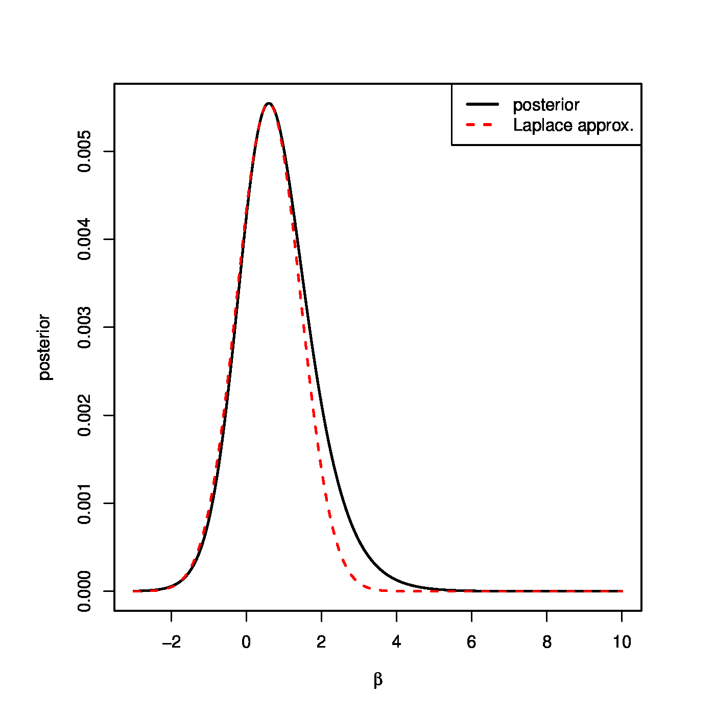
This does not coincide with any standard distribution. But, under appropriate conditions, the posterior distribution is asymptotically normal. This invites a (multivariate) normal approximation to the posterior distribution above. The Laplace's method provides (cf. ).

Laplace approximation to the posterior density of the Bayesian logistic regression parameter.

Laplace's method i) centers the normal approximation at the mode of the posterior, and ii) chooses the covariance to match the curvature of the posterior at the mode. The posterior mode is the location of the maximum of the posterior distribution. The location of this maximum coincides with that of the logarithm of the posterior. The latter is the log-likelihood augmented with a ridge penalty. Hence, the posterior mode, which is taken as the mean of the approximating Gaussian, coincides with the ridge logistic regression estimator. For the covariance of the approximating Gaussian, the logarithm of the posterior is approximated by a second order Taylor series around the posterior mode and limited to second order terms:

[[math]] \begin{eqnarray*} \log[f_{\bbeta}(\bbeta \, | \, \mathbf{Y}, \mathbf{X})] & \propto & \log[f_{\bbeta}(\bbeta \, | \, \mathbf{Y}, \mathbf{X})] \big|_{\bbeta = \hat{\bbeta}_{\mbox{{\tiny MAP}}}} \\ & & + \tfrac{1}{2} (\bbeta - \hat{\bbeta}_{\mbox{{\tiny MAP}}})^{\top} \left. \frac{\partial^2}{\partial \bbeta \partial \bbeta^{\top}} \log[f_{\bbeta}(\bbeta \, | \, \mathbf{Y}, \mathbf{X})] \right|_{\bbeta = \hat{\bbeta}_{\mbox{{\tiny MAP}}}} (\bbeta - \hat{\bbeta}_{\mbox{{\tiny MAP}}})^{\top}, \end{eqnarray*} [[/math]]

in which the first order term cancels as the derivative of [math]f_{\bbeta}(\bbeta \, | \, \mathbf{Y}, \mathbf{X})[/math] with respect to [math]\bbeta[/math] vanishes at the posterior mode -- its maximum. Take the exponential of this approximation and match its arguments to that of a multivariate Gaussian [math]\exp[-\tfrac{1}{2} (\bbeta - \mmu_{\beta})^{\top} \mathbf{\Sigma}_{\bbeta}^{-1} (\bbeta - \mmu_{\beta})][/math]. The covariance of the sought Gaussian approximation is thus the inverse of the Hessian of the negative penalized log-likelihood. Put together the posterior is approximated by:

[[math]] \begin{eqnarray*} \bbeta \, | \, \mathbf{Y}, \mathbf{X} \sim \mathcal{N} [ \hat{\bbeta}_{\mbox{{\tiny MAP}}}, ( \mathbf{\Delta} + \mathbf{X}^{\top} \mathbf{W} \mathbf{X})^{-1} ]. \end{eqnarray*} [[/math]]

The Gaussian approximation is convenient but need not be good. Fortunately, the Bernstein-Von Mises Theorem tells us that it is very accurate when the model is regular, the prior smooth, and the sample size sufficiently large. The quality of the approximation for an artificial example data set is shown in Figure.

Computationally efficient evaluation

High-dimensionally, the IRLS algorithm of the ridge logistic regression estimator can be evaluated computationally efficiently as follows. Hereto, effectively, the problem of penalized likelihood maximization over all [math]\bbeta \in \mathbb{R}^p[/math] is converted into maximization of the same criterion but now over the weights [math]\mbox{diag}(\mathbf{W}) \in \mathbb{R}^n[/math], as those weights are all that are needed for the evaluation of the estimator. The key observations, that enable this conversion, are the following reformulations of the updated linear predictor and the penalty (see Question):

[[math]] \begin{eqnarray} \label{form.compEffRidgeLogistic1} \mathbf{X} \hat{\bbeta} (\lambda) & = & \lambda^{-1} \mathbf{X} \mathbf{X}^{\top} (\lambda^{-1} \mathbf{X} \mathbf{X}^{\top} + \mathbf{W}^{-1})^{-1} \mathbf{Z}, \\ \label{form.compEffRidgeLogistic2} \lambda \| \hat{\bbeta}(\lambda) \|_2^2 & = & \mathbf{Z}^{\top} (\lambda^{-1} \mathbf{X} \mathbf{X}^{\top} + \mathbf{W}^{-1})^{-1} ( \lambda^{-1} \mathbf{X}^{\top} \mathbf{X}^{\top}) (\lambda^{-1} \mathbf{X} \mathbf{X}^{\top} + \mathbf{W}^{-1})^{-1} \mathbf{Z} \end{eqnarray} [[/math]]

Both reformulations hinge upon the Woodbury matrix identity. On one hand, these reformulations avoid the inversion of a [math]p \times p[/math] dimensional matrix (as been shown for the regular ridge regression estimator, see Section Computationally efficient evaluation ). On the other, only the term [math]\lambda^{-1} \mathbf{X} \mathbf{X}^{\top}[/math] in the above expressions involves a matrix multiplication over the [math]p[/math] dimension. Exactly this term is not updated at each iteration of the IRLS algorithm. It can thus be evaluated and stored prior to the first iteration step, and at each iteration be called upon. Furthermore, the remaining quantities updated at each iteration are the weights and the penalized loglikelihood, but those are obtained straightforwardly from the linear predictor and the penalty. The pseudo-code of an efficient version of the IRLS algorithm of the ridge logistic estimator, as has been implemented in the ridgeGLM-function of the porridge-package , thus comprises the following steps:

IRLS algorithm

1. Evaluate and store [math]\lambda^{-1} \mathbf{X} \mathbf{X}^{\top}[/math].
2. Initiate the linear predictor.
3. Update the weights, the adjusted response, the penalized loglikelihood, and the linear predctor.
4. Repeat the previous step until convergence.
5. Evaluate the estimator using the weights from the last iteration.

In the above, convergence refers to no further or a negligible improvement of the penalized loglikelihood. In the final step of this version of the IRLS algorithm, the ridge logistic regression estimator is obtained by:

[[math]] \begin{eqnarray*} \hat{\bbeta} (\lambda) & = & \lambda^{-1} \mathbf{X}^{\top} (\lambda^{-1} \mathbf{X} \mathbf{X}^{\top} + \mathbf{W}^{-1})^{-1} \mathbf{Z}. \end{eqnarray*} [[/math]]

In the above display the weights [math]\mathbf{W}[/math] and adjusted response [math]\mathbf{Z}[/math] are obtained from the last iteraton of the IRLS algorithm's third step. Alternatively, computation efficiency is obtained by the ‘SVD-trick’ (see Question).

Penalty parameter selection

As before the penalty parameter may be chosen through [math]K[/math]-fold cross-validation. For the [math]K=n[/math] case, describe a computationally efficient approximation of the leave-one-out cross-validated loglikelihood. It is based on the exact evaluation of the LOOCV loss, discussed in Section Cross-validation , that avoided resampling. The approach of hinges upon the first-order Taylor expansion of the left-out penalized loglikelihood of the left-out estimate [math]\hat{\bbeta}_{-i} (\lambda)[/math] around [math]\hat{\bbeta} (\lambda)[/math], which yields an approximation of the former:

[[math]] \begin{eqnarray*} \hat{\bbeta}_{-i} (\lambda) & \approx & \hat{\bbeta} (\lambda) - \left( \left. \frac{\partial^2 \mathcal{L}_{-i}^{\mbox{{\tiny pen}}}}{\partial \bbeta \partial \bbeta^{\top}} \right|_{\bbeta = \hat{\bbeta}(\lambda)} \right)^{-1} \left. \frac{\partial \mathcal{L}_{-i}^{\mbox{{\tiny pen}}}}{\partial \bbeta } \right|_{\bbeta = \hat{\bbeta}(\lambda)} \\ & = & \hat{\bbeta} (\lambda) + (\mathbf{X}_{- i, \ast}^{\top} \mathbf{W}_{-i, -i} \mathbf{X}_{- i, \ast} + \lambda \mathbf{I}_{pp})^{-1} \{ \mathbf{X}_{- i, \ast}^{\top} [\mathbf{Y}_{-i} - \vec{\mathbf{g}}^{-1}(\mathbf{X}_{-i, \ast}; \hat{\bbeta}(\lambda))] - \lambda \hat{\bbeta}(\lambda) \}. \end{eqnarray*} [[/math]]

This approximation involves the inverse of a [math]p \times p[/math] dimensional matrix, which amounts to the evaluation of [math]n[/math] such inverses for the LOOCV loss. As in Section Cross-validation this may be avoided. Rewrite both the gradient and the Hessian of the left-out loglikelihood in the approximation of the preceding display:

[[math]] \begin{eqnarray*} & & \hspace{-1.5cm} \mathbf{X}_{-i, \ast}^{\top} \{ \mathbf{Y}_{-i} - \vec{\mathbf{g}}^{-1}(\mathbf{X}_{-i, \ast}; \hat{\bbeta}(\lambda)]\} - \lambda \hat{\bbeta}(\lambda) \\ & = & \mathbf{X}^{\top} \{ \mathbf{Y} - \vec{\mathbf{g}}^{-1}[\mathbf{X}; \hat{\bbeta}(\lambda)]\} - \lambda \hat{\bbeta}(\lambda) - \mathbf{X}_{i, \ast}^{\top} \{Y_{i} - g^{-1}[\mathbf{X}_{i, \ast}; \hat{\bbeta}(\lambda)]\} \\ & = & - \mathbf{X}_{i, \ast}^{\top} \{Y_{i} - g^{-1}[\mathbf{X}_{i, \ast}; \hat{\bbeta}(\lambda)]\} \end{eqnarray*} [[/math]]

and

[[math]] \begin{eqnarray*} (\mathbf{X}_{- i, \ast}^{\top} \mathbf{W}_{-i, -i} \mathbf{X}_{- i, \ast} + \lambda \mathbf{I}_{pp})^{-1} & = & (\mathbf{X}^{\top} \mathbf{W} \mathbf{X} + \lambda \mathbf{I}_{pp})^{-1} + \mathbf{W}_{ii} (\mathbf{X}^{\top} \mathbf{W} \mathbf{X} + \lambda \mathbf{I}_{pp})^{-1} \mathbf{X}_{i, \ast}^{\top} \\ & & \qquad \qquad \qquad \qquad \qquad \quad [ 1 - \mathbf{H}_{ii}(\lambda)]^{-1} \mathbf{X}_{i, \ast} (\mathbf{X}^{\top} \mathbf{W} \mathbf{X} + \lambda \mathbf{I}_{pp})^{-1}, \end{eqnarray*} [[/math]]

where the Woodbury identity has been used and now [math]\mathbf{H}_{ii}(\lambda) = \mathbf{W}_{ii} \mathbf{X}_{i, \ast}(\mathbf{X}^{\top} \mathbf{W} \mathbf{X} + \lambda \mathbf{I}_{pp})^{-1} \mathbf{X}_{i, \ast}^{\top}[/math]. Substitute both in the approximation of the left-out ridge logistic regression estimator and manipulate as in Section Cross-validation to obtain:

[[math]] \begin{eqnarray*} \hat{\bbeta}_{- i}(\lambda) & \approx & \hat{\bbeta}(\lambda) - (\mathbf{X}^{\top} \mathbf{W} \mathbf{X} + \lambda \mathbf{I}_{pp})^{-1} \mathbf{X}_{i, \ast}^{\top} [ 1 - \mathbf{H}_{ii}(\lambda)]^{-1} [ Y_i - g^{-1}(\mathbf{X}_{i, \ast}; \hat{\bbeta}(\lambda)) ]. \end{eqnarray*} [[/math]]

Hence, the leave-one-out cross-validated loglikelihood [math]\sum_{i=1}^n \mathcal{L} [Y_i \, | \, \mathbf{X}_{i, \ast}, \hat{\bbeta}_{-i}(\lambda)][/math] can now be evaluated by means of a single inverse of a [math]p \times p[/math] dimensional matrix and some matrix multiplications. And even this single inversion can be reduced to one of an [math]n \times n[/math]-dimensional matrix when rewritten by means of the Woodbury matrix identity. For the performance of this approximation in terms of accuracy and speed, see .

For general [math]K[/math]-fold cross-validation, computational efficiency is achieved through the same trick as used in Section Cross-validation and reported by . It exploits the fact that the logistic regression parameter only appears in combination with the design matrix, forming the linear predictor, in the loglikelihood. For cross-validation there is thus no need to evaluate the estimator itself. To elaborate on the particulars of the logistic regression case, let [math]\mathcal{G}_1, \ldots, \mathcal{G}_K \subset \{1, \ldots, n\}[/math] be the mutually exclusive and exhaustive [math]K[/math]-fold sample index sets. The linear predictor can then be written as:

[[math]] \begin{eqnarray*} \mathbf{X}_{\mathcal{G}_k, \ast} \hat{\bbeta}_{-\mathcal{G}_k}(\lambda) & = & \lambda^{-1} \mathbf{X}_{\mathcal{G}_k, \ast} \mathbf{X}_{-\mathcal{G}_k, \ast}^{\top} (\lambda^{-1} \mathbf{X}_{-\mathcal{G}_k, \ast} \mathbf{X}_{-\mathcal{G}_k, \ast}^{\top} + \mathbf{W}^{-1})^{-1} \mathbf{Z}, \end{eqnarray*} [[/math]]

which can be verified by means of the Woodbury matrix identity. Furthermore, all matrix products of submatrices of [math]\mathbf{X}[/math] are themselves submatrices of [math]\mathbf{X} \mathbf{X}^{\top}[/math]. Further efficiency is gained if the latter is evaluated before the start of the cross-validation loop. It then only remains to subset [math]\mathbf{X} \mathbf{X}^{\top}[/math] inside this loop.

Application

The ridge logistic regression is used here to explain the status (dead or alive) of ovarian cancer samples at the close of the study from gene expression data at baseline. Data stem from the TCGA study , which measured gene expression by means of sequencing technology. Available are 295 samples with both status and transcriptomic profiles. These profiles are composed of 19990 transcript reads. The sequencing data, being representative of the mRNA transcript count, is heavily skewed. show that a simple transformation of the data prior to model building generally yields a better model than tailor-made approaches. Motivated by this observation the data were -- to accommodate the zero counts -- [math]\mbox{asinh}[/math]-transformed. The logistic regression model is then fitted in ridge penalized fashion, leaving the intercept unpenalized. The ridge penalty parameter is chosen through 10-fold cross-validation minimizing the cross-validated error. R-code, and that for the sequel of this example, is to be found below.

# load libraries
library(glmnet)
library(TCGA2STAT)

# load data
OVdata <- getTCGA(disease="OV", data.type="RNASeq", type="RPKM", clinical=TRUE)
Y      <- as.numeric(OVdata[[3]][,2])
X      <- asinh(data.matrix(OVdata[[3]][,-c(1:3)]))

# start fit
# optimize penalty parameter
cv.fit   <- cv.glmnet(X, Y, alpha=0, family=c("binomial"), 
                            nfolds=10, standardize=FALSE)
optL2    <- cv.fit$lambda.min

# estimate model
glmFit   <- glmnet(X, Y, alpha=0, family=c("binomial"), 
                         lambda=optL2, standardize=FALSE)

# construct linear predictor and predicted probabilities
linPred  <- as.numeric(glmFit$a0 + X %*% glmFit$beta)
predProb <- exp(linPred) / (1+exp(linPred))

# visualize fit
boxplot(linPred ~ Y, pch=20, border="lightblue", col="blue", 
                     ylab="linear predictor", xlab="response", 
                     main="fit")

# evaluate predictive performance
# generate k-folds balanced w.r.t. status
fold     <- 10
folds1   <- rep(1:fold, ceiling(sum(Y)/fold))[1:sum(Y)]
folds0   <- rep(1:fold, ceiling((length(Y)-length(folds1))
                                /fold))[1:(length(Y)-length(folds1))]
shuffle1 <- sample(1:length(folds1), length(folds1))
shuffle0 <- sample(1:length(folds0), length(folds0))
folds1   <- split(shuffle1, as.factor(folds1))
folds0   <- split(shuffle0, as.factor(folds0))
folds    <- list()
for (f in 1:fold){
	folds[[f]] <- c(which(Y==1)[folds1[[f]]], which(Y==0)[folds0[[f]]])
}
for (f in 1:fold){
	print(sum(Y[folds[[f]]]))
}

# build model
pred2obsL2 <- matrix(nrow=0, ncol=4)
colnames(pred2obsL2) <- c("optLambda", "linPred", "predProb", "obs")
for (f in 1:length(folds)){
	print(f)
	cv.fit     <- cv.glmnet(X[-folds[[f]],], Y[-folds[[f]]], alpha=0, 
	                        family=c("binomial"), nfolds=10, standardize=FALSE)
	optL2      <- cv.fit$lambda.min
	glmFit     <- glmnet(X[-folds[[f]],], Y[-folds[[f]]], alpha=0, 
	                     family=c("binomial"), lambda=optL2, standardize=FALSE)
	linPred    <- glmFit$a0 + X[folds[[f]],,drop=FALSE] %*% glmFit$beta
	predProb   <- exp(linPred) / (1+exp(linPred))
	pred2obsL2 <- rbind(pred2obsL2, cbind(optL2, linPred, predProb, Y[folds[[f]]]))
}

# visualize fit
boxplot(pred2obsL2[,3] ~ pred2obsL2[,4], pch=20, border="lightblue", col="blue", 
                                         ylab="linear predictor", xlab="response", 
                                         main="prediction")

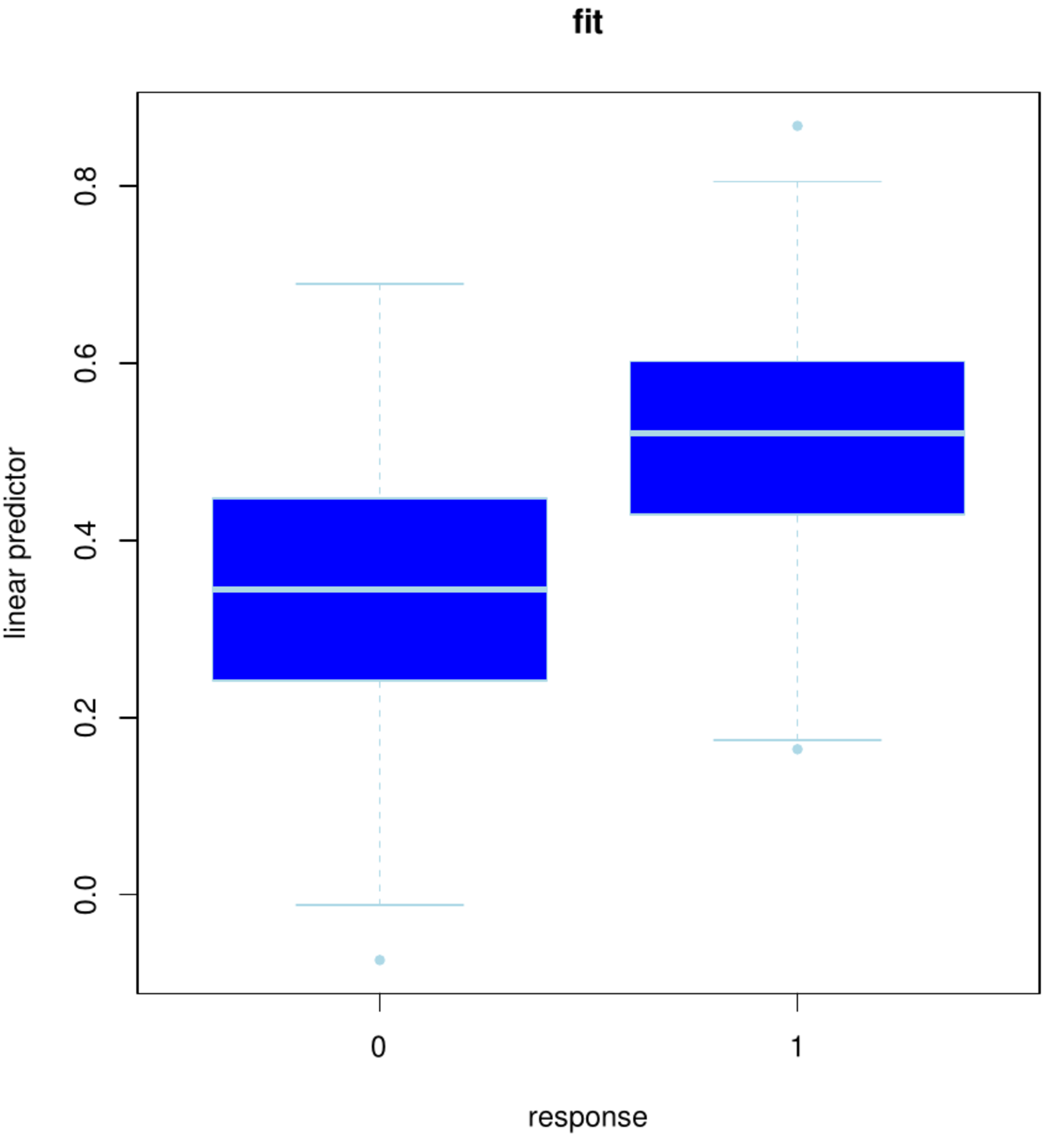
The fit of the resulting model is studied. Hereto the fitted linear predictor [math]\mathbf{X} \hat{\bbeta}(\lambda_{\mbox{\tiny opt}})[/math] is plotted against the status (Figure, left panel). The plot shows some overlap between the boxes, but also a clear separation. The latter suggests gene expression at baseline thus enables us to distinguish surviving from the to-be-diseased ovarian cancer patients. Ideally, a decision rule based on the linear predictor can be formulated to predict an individual's outcome.

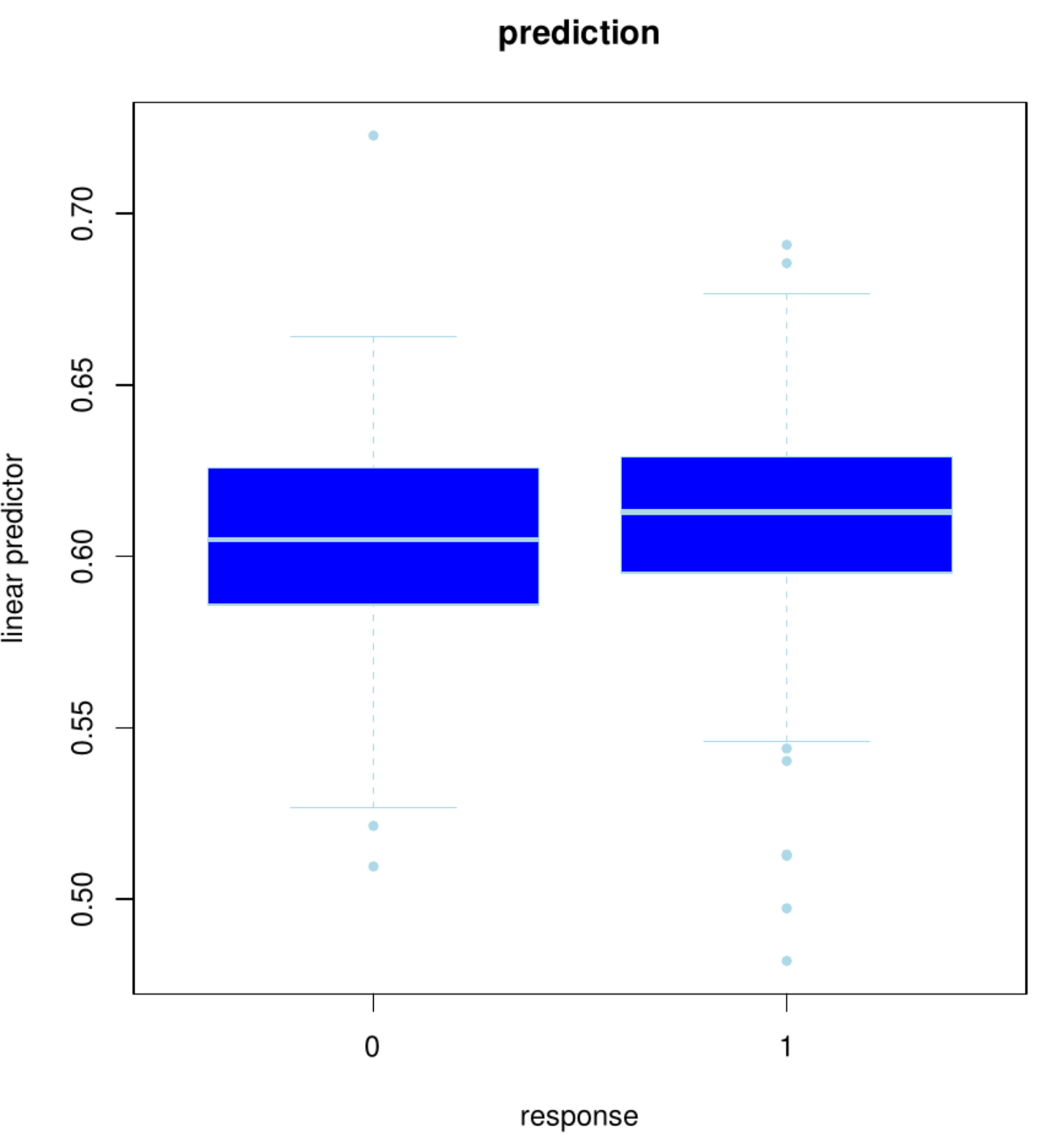
Left panel: Box plot of the status vs. the fitted linear predictor using the full data set. Right panel: Box plot of the status vs. the linear prediction in the left-out samples of the 10 folds.

The fit, however, is evaluated on the samples that have been used to build the model. This gives no insight on the model's predictive performance on novel samples. A replication of the study is generally costly and comparable data sets need not be at hand. A common workaround is to evaluate the predictive performance on the same data . This requires to put several samples aside for performance evaluation while the remainder is used for model building. The left-out sample may accidently be chosen to yield an exaggerated (either dramatically poor or overly optimistic) performance. This is avoided through the repetition of this exercise, leaving (groups of) samples out one at the time. The left-out performance evaluations are then averaged and believed to be representative of the predictive performance of the model on novel samples. Note that, effectively, as the model building involves cross-validation and so does the performance evaluation, a double cross-validation loop is applied. This procedure is applied with a ten-fold split in both loops. Denote the outer folds by [math]f = 1, \ldots, 10[/math]. Then, [math]\mathbf{X}_{f}[/math] and [math]\mathbf{X}_{-f}[/math] represent the design matrix of the samples comprising fold [math]f[/math] and that of the remaining samples, respectively. Define [math]\mathbf{Y}_{f}[/math] and [math]\mathbf{Y}_{-f}[/math] similarly. The linear prediction for the left-out fold [math]f[/math] is then [math]\mathbf{X}_{f} \hat{\bbeta}_{-f} (\lambda_{\mbox{{\tiny opt, -f}}})[/math]. For reference to the fit, this is compared to [math]\mathbf{Y}_{f}[/math] visually by means of a boxplot as used above (see Figure, right panel). The boxes overlap almost perfectly. Hence, little to nothing remains of the predictive power suggested by the boxplot of the fit. The fit may thus give a reasonable description of the data at hand, but it extrapolates poorly to new samples.

Conclusion

To deal with response variables other than continuous ones, ridge logistic regression was discussed. High-dimensionally, the empirical identifiability problem then persists. Again, penalization came to the rescue: the ridge penalty may be combined with other link functions than the identity. Properties of ridge regression were shown to carry over to its logistic equivalent.

General References

van Wieringen, Wessel N. (2021). "Lecture notes on ridge regression". arXiv:1509.09169 [stat.ME].

References

- Hosmer Jr, D. W., Lemeshow, S., and Sturdivant, R. X. (2013).Applied Logistic Regression, volume 398.John Wiley & Sons
- Schaefer, R. L., Roi, L. D., and Wolfe, R. A. (1984).A ridge logistic estimator.Communications in Statistics: Theory and Methods, 13(1), 99--113
- Le Cessie, S. and Van Houwelingen, J. C. (1992).Ridge estimators in logistic regression.Applied Statistics, 41(1), 191--201
- Bishop, C. M. (2006).Pattern Recognition and Machine Learning.Springer
- van der Vaart, A. W. (2000).Asymptotic Statistics, volume 3.Cambridge University Press
- van Wieringen, W. and Aflakparast, M. (2021).porridge: Ridge-Type Estimation of a Potpourri of Models.R package version 0.2.1
- 7.0 7.1 7.2 Meijer, R. J. and Goeman, J. J. (2013).Efficient approximate k-fold and leave-one-out cross-validation for ridge regression.Biometrical Journal, 55(2), 141--155
- van de Wiel, M. A., van Nee, M. M., and Rauschenberger, A. (2021).Fast cross-validation for multi-penalty ridge regression.Journal of Computational and Graphical Statistics, (just-accepted), 1--31
- Cancer Genome Atlas Network (2011).Integrated genomic analyses of ovarian carcinoma.Nature, 474(7353), 609--615
- Zwiener, I., Frisch, B., and Binder, H. (2014).Transforming RNA-seq data to improve the performance of prognostic gene signatures.PloS one, 9(1), e85150
- Subramanian, J. and Simon, R. (2010).Gene expression--based prognostic signatures in lung cancer: ready for clinical use?Journal of the National Cancer Institute, 102(7), 464--474