guide:Ec62e49ef0: Difference between revisions
No edit summary |
mNo edit summary |
||
| (One intermediate revision by one other user not shown) | |||
| Line 1: | Line 1: | ||
<div class="d-none"><math> | |||
\newcommand{\NA}{{\rm NA}} | |||
\newcommand{\mat}[1]{{\bf#1}} | |||
\newcommand{\exref}[1]{\ref{##1}} | |||
\newcommand{\secstoprocess}{\all} | |||
\newcommand{\NA}{{\rm NA}} | |||
\newcommand{\mathds}{\mathbb}</math></div> | |||
In this section we consider the continuous version of the problem posed in the previous section: How are sums of independent random variables distributed? | |||
===Convolutions=== | |||
{{defncard|label=|id=|Let <math>X</math> and <math>Y</math> be two continuous random variables with density | |||
functions <math>f(x)</math> and <math>g(y)</math>, respectively. Assume that both <math>f(x)</math> and <math>g(y)</math> are defined for | |||
all real numbers. Then the ''convolution'' <math>f*g</math> of <math>f</math> and <math>g</math> is the function given by | |||
<math display="block"> | |||
\begin{eqnarray*} (f*g)(z) &=& \int_{-\infty}^{+\infty} f(z - y) g(y)\,dy \\ | |||
&=& \int_{-\infty}^{+\infty} g(z - x) f(x)\, dx\ . | |||
\end{eqnarray*} | |||
</math> | |||
}} | |||
This definition is analogous to the definition, given in [[guide:4c79910a98|Sums of Discrete Random Variables]], of the convolution of two distribution functions. Thus it should not be surprising that if <math>X</math> and <math>Y</math> are independent, then the density of their sum is the convolution of their densities. | |||
This fact is stated as a theorem below, and its proof is left as an exercise (see [[exercise:30fa15e033 |Exercise]]). | |||
{{proofcard|Theorem|theorem-1|Let <math>X</math> and <math>Y</math> be two independent random variables with density functions | |||
<math>f_X(x)</math> and <math>f_Y(y)</math> defined for all <math>x</math>. Then the sum <math>Z = X + Y</math> is a random variable with | |||
density function <math>f_Z(z)</math>, where <math>f_Z</math> is the convolution of <math>f_X</math> and <math>f_Y</math>.|}} | |||
To get a better understanding of this important result, we will look at some examples. | |||
===Sum of Two Independent Uniform Random Variables=== | |||
<span id="exam 7.6"/> | |||
'''Example''' | |||
Suppose we choose independently two numbers at random from the interval | |||
<math>[0,1]</math> with uniform probability density. What is the | |||
density of their sum? | |||
Let <math>X</math> and <math>Y</math> be random variables describing our choices and <math>Z = X + Y</math> | |||
their sum. Then we have | |||
<math display="block"> | |||
f_X(x) = f_Y(x) = \left \{ \begin{array}{ll} | |||
1 & \;\mbox{if $0 \leq x \leq 1$,} \\ | |||
0 & \;\mbox{otherwise;} | |||
\end{array} | |||
\right. | |||
</math> | |||
and the density function for the sum is given by | |||
<math display="block"> | |||
f_Z(z) = \int_{-\infty}^{+\infty} f_X(z - y) f_Y(y)\,dy\ . | |||
</math> | |||
Since <math>f_Y(y) = 1</math> if <math>0 \leq y \leq 1</math> and 0 otherwise, this becomes | |||
<math display="block"> | |||
f_Z(z) = \int_0^1 f_X(z - y)\,dy\ . | |||
</math> | |||
Now the integrand is 0 unless <math>0 \leq z - y \leq 1</math> (i.e., unless <math>z - 1 \leq y | |||
\leq z</math>) and then it is 1. So if <math>0 \leq z \leq 1</math>, we have | |||
<math display="block"> | |||
f_Z(z) = \int_0^z \, dy = z\ , | |||
</math> | |||
while if <math>1 < z \leq 2</math>, we have | |||
<math display="block"> | |||
f_Z(z) = \int_{z - 1}^1\, dy = 2 - z\ , | |||
</math> | |||
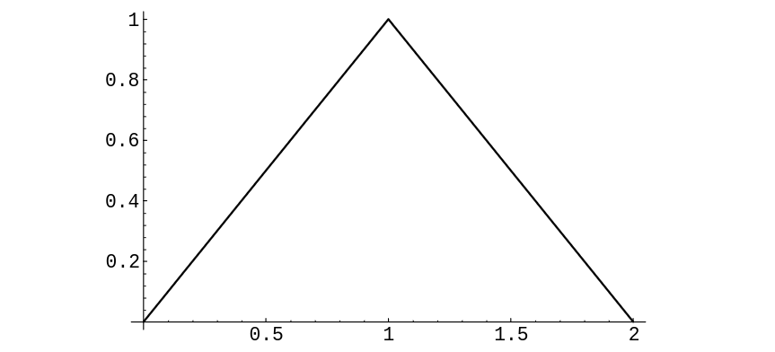
and if <math>z < 0</math> or <math>z > 2</math> we have <math>f_Z(z) = 0</math> (see [[#fig 7.5|Figure]]). Hence, | |||
<math display="block"> | |||
f_Z(z) = \left \{ \begin{array}{ll} | |||
z, & \;\mbox{if $0 \leq z \leq 1,$} \\ | |||
2-z, & \;\mbox{if $1 < z \leq 2,$} \\ | |||
0, & \;\mbox{otherwise.} | |||
\end{array} | |||
\right. | |||
</math> | |||
<div id="fig 7.5" class="d-flex justify-content-center"> | |||
[[File:guide_e6d15_PSfig7-5.png | 400px | thumb |Convolution of two uniform densities. ]] | |||
</div> | |||
Note that this result agrees with that of [[guide:A070937c41#exam 2.1.4.5 |Example]]. | |||
===Sum of Two Independent Exponential Random Variables=== | |||
<span id="exam 7.7"/> | |||
'''Example''' | |||
Suppose we choose two numbers at random from the interval <math>[0,\infty)</math> with | |||
an ''exponential'' density with parameter <math>\lambda</math>. | |||
What is the density of their sum? | |||
Let <math>X</math>, <math>Y</math>, and <math>Z = X + Y</math> denote the relevant random variables, and | |||
<math>f_X</math>, <math>f_Y</math>, and <math>f_Z</math> their densities. Then | |||
<math display="block"> | |||
f_X(x) = f_Y(x) = \left \{ \begin{array}{ll} | |||
\lambda e^{-\lambda x}, & \;\mbox{if $x \geq 0$},\\ | |||
0, & \;\mbox{otherwise;} | |||
\end{array} | |||
\right. | |||
</math> | |||
and so, if <math>z > 0</math>, | |||
<math display="block"> | |||
\begin{eqnarray*} | |||
f_Z(z) &=& \int_{-\infty}^{+\infty} f_X(z - y) f_Y(y)\, dy \\ | |||
&=& \int_0^z \lambda e^{-\lambda(z - y)} \lambda e^{-\lambda y}\, dy \\ | |||
&=& \int_0^z \lambda^2 e^{-\lambda z}\, dy \\ | |||
&=& \lambda^2 z e^{-\lambda z},\\ | |||
\end{eqnarray*} | |||
</math> | |||
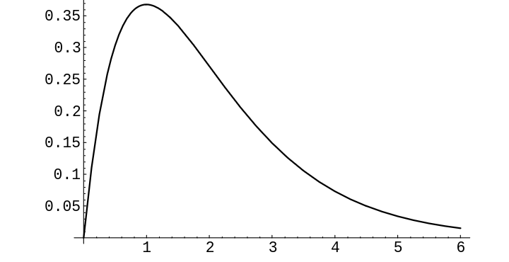
while if <math>z < 0</math>, <math>f_Z(z) = 0</math> (see [[#fig 7.6|Figure]]). Hence, | |||
<div id="fig 7.6" class="d-flex justify-content-center"> | |||
[[File:guide_e6d15_PSfig7-6.png | 400px | thumb | Convolution of two exponential densities with <math>\lambda = 1</math>. ]] | |||
</div> | |||
<math display="block"> | |||
f_Z(z) = \left \{ \begin{array}{ll} | |||
\lambda^2 z e^{-\lambda z}, | |||
& \;\mbox{if $z \geq 0$},\\ | |||
0, & \;\mbox{otherwise.} | |||
\end{array} | |||
\right. | |||
</math> | |||
===Sum of Two Independent Normal Random Variables=== | |||
<span id="exam 7.8"/> | |||
'''Example''' | |||
It is an interesting and important fact that the convolution of two normal | |||
densities with means <math>\mu_1</math> and <math>\mu_2</math> and variances <math>\sigma_1</math> and <math>\sigma_2</math> is | |||
again a normal density, with mean <math>\mu_1 + \mu_2</math> and variance <math>\sigma_1^2 + \sigma_2^2</math>. | |||
We will show this in the special case that both random variables are standard normal. | |||
The general case can be done in the same way, but the calculation is messier. Another | |||
way to show the general result is given in [[guide:31815919f9#exam 10.3.3 |Example]]. | |||
Suppose <math>X</math> and <math>Y</math> are two independent random variables, each with the standard ''normal'' density (see [[guide:D26a5cb8f7#exam 5.16 |Example]]). | |||
We have | |||
<math display="block"> | |||
f_X(x) = f_Y(y) = \frac 1{\sqrt{2\pi}} e^{-x^2/2}\ , | |||
</math> | |||
and so | |||
<math display="block"> | |||
\begin{eqnarray*} | |||
f_Z(z) &=& f_X * f_Y(z) \\ | |||
&=& \frac 1{2\pi} \int_{-\infty}^{+\infty} e^{-(z - | |||
y)^2/2} e^{-y^2/2}\, dy \\ | |||
&=& \frac 1{2\pi} e^{-z^2/4} \int_{-\infty}^{+\infty} e^{-(y - z/2)^2}\, | |||
dy \\ | |||
&=& \frac 1{2\pi} e^{-z^2/4}\sqrt {\pi} \biggl[\frac 1{\sqrt {\pi}}\int_{-\infty}^\infty | |||
e^{-(y-z/2)^2}\,dy\ \biggr]\ .\\ | |||
\end{eqnarray*} | |||
</math> | |||
The expression in the brackets equals 1, since it is the integral of the normal density | |||
function with <math>\mu = 0</math> and <math>\sigma = \sqrt 2</math>. So, we have | |||
<math display="block"> | |||
f_Z(z) = \frac 1{\sqrt{4\pi}} e^{-z^2/4}\ . | |||
</math> | |||
===Sum of Two Independent Cauchy Random Variables=== | |||
<span id="exam 7.9"/> | |||
'''Example''' | |||
Choose two numbers at random from the interval | |||
<math>(-\infty,+\infty)</math> with the Cauchy density | |||
with parameter <math>a = 1</math> (see [[guide:D26a5cb8f7#exam 5.20 |Example]]). Then | |||
<math display="block"> | |||
f_X(x) = f_Y(x) = \frac 1{\pi(1 + x^2)}\ , | |||
</math> | |||
and <math>Z = X + Y</math> has density | |||
<math display="block"> | |||
f_Z(z) = \frac 1{\pi^2} \int_{-\infty}^{+\infty} \frac {1}{1 + (z - y)^2} \frac | |||
{1}{1 + y^2} \, dy\ . | |||
</math> | |||
This integral requires some effort, and we give here only the result | |||
(see Section \ref{sec 10.3}, or Dwass<ref group="Notes" >M. Dwass, “On the Convolution of Cauchy | |||
Distributions,” ''American Mathematical Monthly,'' vol. 92, no. 1, (1985), | |||
pp. 55--57; see also R. Nelson, letters to the Editor, ibid., p. 679.</ref>): | |||
<math display="block"> | |||
f_Z(z) = \frac {2}{\pi(4 + z^2)}\ . | |||
</math> | |||
Now, suppose that we ask for the density function of the ''average'' | |||
<math display="block"> | |||
A = (1/2)(X + Y) | |||
</math> | |||
of <math>X</math> and <math>Y</math>. Then <math>A = (1/2)Z</math>. [[exercise:242a63cd0b|Exercise]] shows that if <math>U</math> and <math>V</math> are two continuous random variables with density functions | |||
<math>f_U(x)</math> and <math>f_V(x)</math>, respectively, and if <math>V = aU</math>, then | |||
<math display="block"> | |||
f_V(x) = \biggl(\frac 1a\biggr)f_U\biggl(\frac xa\biggr)\ . | |||
</math> | |||
Thus, we have | |||
<math display="block"> | |||
f_A(z) = 2f_Z(2z) = \frac 1{\pi(1 + z^2)}\ . | |||
</math> | |||
Hence, the density function for the average of two random variables, each | |||
having a Cauchy density, is again a random variable with a Cauchy density; this | |||
remarkable property is a peculiarity of the Cauchy density. One consequence of | |||
this is if the error in a certain measurement process had a Cauchy | |||
density and you averaged a number of measurements, the average could not be | |||
expected to be any more accurate than any one of your individual measurements! | |||
===Rayleigh Density=== | |||
<span id="exam 7.10"/> | |||
'''Example''' | |||
Suppose <math>X</math> and <math>Y</math> are two independent standard normal random variables. | |||
Now suppose we locate a point <math>P</math> in the <math>xy</math>-plane with coordinates <math>(X,Y)</math> and | |||
ask: What is the density of the square of the distance of <math>P</math> from the origin? | |||
(We have already simulated this problem in [[guide:D26a5cb8f7#exam 5.19 |Example]].) Here, with the preceding | |||
notation, we have | |||
<math display="block"> | |||
f_X(x) = f_Y(x) = \frac 1{\sqrt{2\pi}} e^{-x^2/2}\ . | |||
</math> | |||
Moreover, if <math>X^2</math> denotes the square of <math>X</math>, then (see [[guide:D26a5cb8f7#thm 5.1 |Theorem]] and the | |||
discussion following) | |||
<math display="block"> | |||
\begin{eqnarray*} | |||
f_{X^2}(r) &=& \left \{ \begin{array}{ll} | |||
\frac{1}{2\sqrt r} (f_X(\sqrt r) + f_X(-\sqrt r)) & \;\mbox{if $r > 0,$} \\ | |||
0 & \;\mbox{otherwise.} | |||
\end{array} | |||
\right. \\ | |||
&=& \left \{ \begin{array}{ll} | |||
\frac{1}{\sqrt {2 \pi r}} (e^{-r/2}) & \;\mbox{if $r > 0,$} \\ | |||
0 & \;\mbox{otherwise.} | |||
\end{array} | |||
\right. \\ | |||
\end{eqnarray*} | |||
</math> | |||
This is a gamma density with <math>\lambda = 1/2</math>, <math>\beta = 1/2</math> (see | |||
[[#exam 7.7 |Example]]). Now let <math>R^2 = X^2 + Y^2</math>. Then | |||
<math display="block"> | |||
\begin{eqnarray*} | |||
f_{R^2}(r) &=& \int_{-\infty}^{+\infty} f_{X^2}(r - s) f_{Y^2}(s)\, ds \\ | |||
&=& \frac 1{4\pi} \int_{-\infty}^{+\infty} e^{-(r - s)/2} | |||
{\frac{r-s}{2}}^{-1/2} e^{-s} {\frac{s}{2}}^{-1/2}\, ds\ , \\ | |||
&=& \left \{\begin{array}{ll} | |||
{\frac {1}{2}} e^{-r^2/2}, & \;\mbox{if $r \geq 0,$} \\ | |||
0, & \;\mbox{otherwise.} | |||
\end{array} | |||
\right. | |||
\end{eqnarray*} | |||
</math> | |||
Hence, <math>R^2</math> has a gamma density with <math>\lambda = 1/2</math>, <math>\beta = 1</math>. We can | |||
interpret this result as giving the density for the square of the distance | |||
of <math>P</math> from the center of a target if its coordinates are normally distributed. | |||
The density of the random variable <math>R</math> is obtained from that of <math>R^2</math> in the | |||
usual way (see [[guide:D26a5cb8f7#thm 5.1 |Theorem]]), and we find | |||
<math display="block"> | |||
f_R(r) = \left \{ \begin{array}{ll} | |||
\frac 12 e^{-r^2/2} \cdot 2r = re^{-r^2/2}, | |||
& \;\mbox{if $r \geq 0,$} \\ | |||
0, & \;\mbox{otherwise.} | |||
\end{array} | |||
\right. | |||
</math> | |||
Physicists will recognize this as a Rayleigh density. Our | |||
result here agrees with our simulation in [[guide:D26a5cb8f7#exam 5.19 |Example]]. | |||
===Chi-Squared Density=== | |||
More generally, the same method shows that the sum of the squares of <math>n</math> | |||
independent normally distributed random variables with mean 0 and standard | |||
deviation 1 has a gamma density with <math>\lambda = 1/2</math> and <math>\beta = n/2</math>. Such a | |||
density is called a ''chi-squared density'' with <math>n</math> degrees of freedom. This | |||
density was introduced in Chapter [[guide:A618cf4c07|Distributions and Densities]]. In [[guide:D26a5cb8f7#exam 5.20 |Example]], we | |||
used this density to test the hypothesis that two traits were independent. | |||
Another important use of the chi-squared density is in comparing experimental data | |||
with a theoretical discrete distribution, to see whether the data supports the | |||
theoretical model. More specifically, suppose that we have an experiment with a | |||
finite set of outcomes. If the set of outcomes is countable, we group them into | |||
finitely many sets of outcomes. We propose a theoretical distribution which we think | |||
will model the experiment well. We obtain some data by repeating the experiment a | |||
number of times. Now we wish to check how well the theoretical distribution fits the | |||
data. | |||
Let <math>X</math> be the random variable which represents a theoretical outcome in the model | |||
of the experiment, and let <math>m(x)</math> be the distribution function of <math>X</math>. In a manner | |||
similar to what was done in [[guide:D26a5cb8f7#exam 5.20 |Example]], we calculate the value of the | |||
expression | |||
<math display="block"> | |||
V = \sum_x \frac{(o_x - n \cdot m(x))^2}{n \cdot m(x)}\ , | |||
</math> | |||
where the sum runs over all possible outcomes <math>x</math>, <math>n</math> is the number of data | |||
points, and <math>o_x</math> denotes the number of outcomes of type <math>x</math> observed | |||
in the data. Then for moderate or large values of <math>n</math>, the quantity <math>V</math> is | |||
approximately chi-squared distributed, with <math>\nu - 1</math> degrees of freedom, where | |||
<math>\nu</math> represents the number of possible outcomes. The proof of this is beyond the | |||
scope of this book, but we will illustrate the reasonableness of this statement in | |||
the next example. If the value of <math>V</math> is very large, when compared with the | |||
appropriate chi-squared density function, then we would tend to reject the hypothesis | |||
that the model is an appropriate one for the experiment at hand. We now give an | |||
example of this procedure. | |||
'''Example''' | |||
Suppose we are given a single die. We wish to test the hypothesis that the die is fair. Thus, our theoretical distribution is the uniform distribution on the integers between 1 and 6. So, if we roll the die <math>n</math> times, the expected number of data points of each type is <math>n/6</math>. Thus, if <math>o_i</math> denotes the actual number of data points of type <math>i</math>, for <math>1 \le i \le 6</math>, then the expression | |||
<math display="block"> | |||
V = \sum_{i = 1}^6 \frac{(o_i - n/6)^2}{n/6} | |||
</math> | |||
is approximately chi-squared distributed with 5 degrees of freedom. | |||
Now suppose that we actually roll the die 60 times and obtain the | |||
data in [[#table 7.1 |Table]]. | |||
<span id="table 7.1"/> | |||
{|class="table" | |||
|+ Observed data. | |||
|- | |||
|Outcome || Observed Frequency | |||
|- | |||
|1 || 15 | |||
|- | |||
|2 || 8 | |||
|- | |||
|3 || 7 | |||
|- | |||
|4 || 5 | |||
|- | |||
|5 || 7 | |||
|- | |||
|6 || 18 | |||
|} | |||
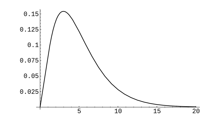
If we calculate <math>V</math> for this data, we obtain the value 13.6. The graph of the | |||
chi-squared density with 5 degrees of freedom is shown in [[#fig 7.7|Figure]]. One | |||
sees that values as large as 13.6 are rarely taken on by <math>V</math> if the die is fair, so we | |||
would reject the hypothesis that the die is fair. (When using this test, a | |||
statistician will reject the hypothesis if the data gives a value of <math>V</math> which is | |||
larger than 95% of the values one would expect to obtain if the hypothesis is true.) | |||
<div id="fig 7.7" class="d-flex justify-content-center"> | |||
[[File:guide_e6d15_PSfig7-7.png | 400px | thumb | Chi-squared density with 5 degrees of freedom. ]] | |||
</div> | |||
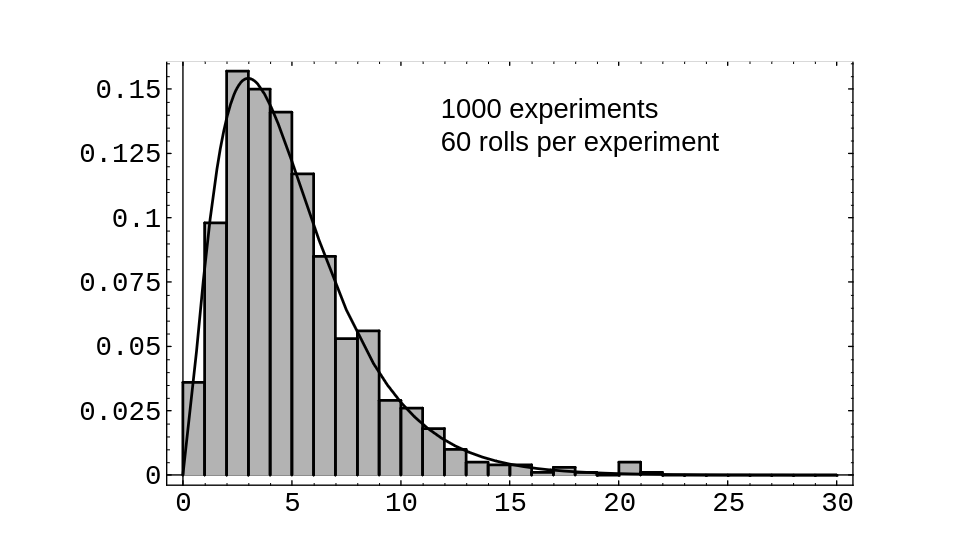
In [[#fig 7.8|Figure]], we show the results of rolling a die 60 times, then | |||
calculating <math>V</math>, and then repeating this experiment 1000 times. The program that performs | |||
these calculations is called ''' DieTest'''. We | |||
have superimposed the chi-squared density with 5 degrees of freedom; one can see | |||
that the data values fit the curve fairly well, which supports the statement | |||
that the chi-squared density is the correct one to use. | |||
<div id="fig 7.8" class="d-flex justify-content-center"> | |||
[[File:guide_e6d15_PSfig7-8.png | 400px | thumb | Rolling a fair die. ]] | |||
</div> | |||
So far we have looked at several important special cases for which the | |||
convolution integral can be evaluated explicitly. In general, the convolution | |||
of two continuous densities cannot be evaluated explicitly, and we must resort | |||
to numerical methods. Fortunately, these prove to be remarkably effective, at | |||
least for bounded densities. | |||
===Independent Trials=== | |||
We now consider briefly the distribution of the sum of <math>n</math> independent random | |||
variables, all having the same density function. If <math>X_1</math>, <math>X_2</math>, \dots, <math>X_n</math> | |||
are these random variables and <math>S_n = X_1 + X_2 +\cdots+ X_n</math> is their sum, then we | |||
will have | |||
<math display="block"> | |||
f_{S_n}(x) = \left( f_{X_1} * f_{X_2} *\cdots* f_{X_n} \right)(x)\ , | |||
</math> | |||
where the right-hand side is an <math>n</math>-fold convolution. It is possible to | |||
calculate this density for general values of <math>n</math> in certain simple cases. | |||
<span id="exam 7.12"/> | |||
'''Example''' | |||
Suppose the <math>X_i</math> are uniformly distributed on the interval | |||
<math>[0,1]</math>. Then | |||
<math display="block"> | |||
f_{X_i}(x) = \left \{ \begin{array}{ll} | |||
1, & \;\mbox{if $0 \leq x \leq 1,$} \\ | |||
0, & \;\mbox{otherwise,} | |||
\end{array} | |||
\right. | |||
</math> | |||
and <math>f_{S_n}(x)</math> is given by the formula<ref group="Notes" >J. B. Uspensky, | |||
'' Introduction to Mathematical Probability'' (New York: McGraw-Hill, 1937), | |||
p. 277.</ref> | |||
<math display="block"> | |||
f_{S_n}(x) = \left \{ \begin{array}{ll} | |||
\frac 1{(n - 1)!} \sum_{0 \leq j \leq x} (-1)^j | |||
{ n \choose j} (x - j)^{n - 1}, & \;\mbox{if $0 < x < n,$} \\ | |||
0, & \;\mbox{otherwise.} | |||
\end{array} | |||
\right. | |||
</math> | |||
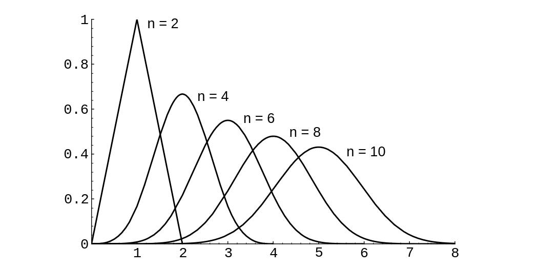
The density <math>f_{S_n}(x)</math> for <math>n = 2</math>, 4, 6, 8, 10 is shown in [[#fig 7.9|Figure]]. | |||
<div id="Convolution of <math>n</math> uniform densities." class="d-flex justify-content-center"> | |||
[[File:guide_e6d15_PSfig7-9.png | 400px | thumb | Convolution of <math>n</math> uniform densities.]] | |||
</div> | |||
If the <math>X_i</math> are distributed normally, with mean 0 | |||
and variance 1, then (cf. [[#exam 7.8 |Example]]) | |||
<math display="block"> | |||
f_{X_i}(x) = \frac 1{\sqrt{2\pi}} e^{-x^2/2}\ , | |||
</math> | |||
and | |||
<math display="block"> | |||
f_{S_n}(x) = \frac 1{\sqrt{2\pi n}} e^{-x^2/2n}\ . | |||
</math> | |||
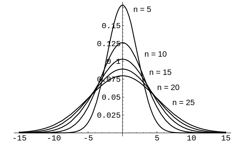
Here the density <math>f_{S_n}</math> for <math>n = 5</math>, 10, 15, 20, 25 is shown in [[#fig 7.10|Figure]]. | |||
<div id="fig 7.10" class="d-flex justify-content-center"> | |||
[[File:guide_e6d15_PSfig7-10.png | 400px | thumb |Convolution of <math>n</math> standard normal densities. ]] | |||
</div> | |||
If the <math>X_i</math> are all exponentially distributed, | |||
with mean <math>1/\lambda</math>, then | |||
<math display="block"> | |||
f_{X_i}(x) = \lambda e^{-\lambda x}\ , | |||
</math> | |||
and | |||
<math display="block"> | |||
f_{S_n}(x) = \frac {\lambda e^{-\lambda x}(\lambda x)^{n - 1}}{(n - 1)!}\ . | |||
</math> | |||
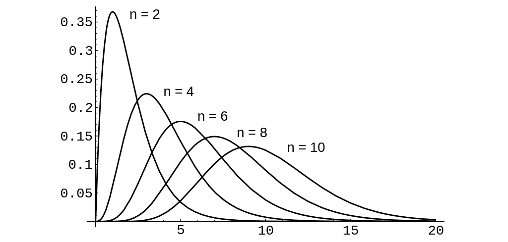
In this case the density <math>f_{S_n}</math> for <math>n = 2</math>, 4, 6, 8, 10 is shown in | |||
[[#fig 7.11|Figure]]. | |||
<div id="fig 7.11" class="d-flex justify-content-center"> | |||
[[File:guide_e6d15_PSfig7-11.png | 400px | thumb | Convolution of <math>n</math> exponential densities with <math>\lambda = 1</math>. ]] | |||
</div> | |||
==General references== | |||
{{cite web |url=https://math.dartmouth.edu/~prob/prob/prob.pdf |title=Grinstead and Snell’s Introduction to Probability |last=Doyle |first=Peter G.|date=2006 |access-date=June 6, 2024}} | |||
==Notes== | |||
{{Reflist|group=Notes}} | |||
Latest revision as of 02:18, 11 June 2024
In this section we consider the continuous version of the problem posed in the previous section: How are sums of independent random variables distributed?
Convolutions
Let [math]X[/math] and [math]Y[/math] be two continuous random variables with density functions [math]f(x)[/math] and [math]g(y)[/math], respectively. Assume that both [math]f(x)[/math] and [math]g(y)[/math] are defined for all real numbers. Then the convolution [math]f*g[/math] of [math]f[/math] and [math]g[/math] is the function given by
This definition is analogous to the definition, given in Sums of Discrete Random Variables, of the convolution of two distribution functions. Thus it should not be surprising that if [math]X[/math] and [math]Y[/math] are independent, then the density of their sum is the convolution of their densities. This fact is stated as a theorem below, and its proof is left as an exercise (see Exercise).
Let [math]X[/math] and [math]Y[/math] be two independent random variables with density functions [math]f_X(x)[/math] and [math]f_Y(y)[/math] defined for all [math]x[/math]. Then the sum [math]Z = X + Y[/math] is a random variable with density function [math]f_Z(z)[/math], where [math]f_Z[/math] is the convolution of [math]f_X[/math] and [math]f_Y[/math].
To get a better understanding of this important result, we will look at some examples.
Sum of Two Independent Uniform Random Variables
Example Suppose we choose independently two numbers at random from the interval [math][0,1][/math] with uniform probability density. What is the density of their sum? Let [math]X[/math] and [math]Y[/math] be random variables describing our choices and [math]Z = X + Y[/math] their sum. Then we have
and the density function for the sum is given by
Since [math]f_Y(y) = 1[/math] if [math]0 \leq y \leq 1[/math] and 0 otherwise, this becomes
Now the integrand is 0 unless [math]0 \leq z - y \leq 1[/math] (i.e., unless [math]z - 1 \leq y \leq z[/math]) and then it is 1. So if [math]0 \leq z \leq 1[/math], we have
while if [math]1 \lt z \leq 2[/math], we have
and if [math]z \lt 0[/math] or [math]z \gt 2[/math] we have [math]f_Z(z) = 0[/math] (see Figure). Hence,
Note that this result agrees with that of Example.
Sum of Two Independent Exponential Random Variables
Example Suppose we choose two numbers at random from the interval [math][0,\infty)[/math] with an exponential density with parameter [math]\lambda[/math]. What is the density of their sum? Let [math]X[/math], [math]Y[/math], and [math]Z = X + Y[/math] denote the relevant random variables, and [math]f_X[/math], [math]f_Y[/math], and [math]f_Z[/math] their densities. Then
and so, if [math]z \gt 0[/math],
while if [math]z \lt 0[/math], [math]f_Z(z) = 0[/math] (see Figure). Hence,
Sum of Two Independent Normal Random Variables
Example It is an interesting and important fact that the convolution of two normal densities with means [math]\mu_1[/math] and [math]\mu_2[/math] and variances [math]\sigma_1[/math] and [math]\sigma_2[/math] is again a normal density, with mean [math]\mu_1 + \mu_2[/math] and variance [math]\sigma_1^2 + \sigma_2^2[/math]. We will show this in the special case that both random variables are standard normal. The general case can be done in the same way, but the calculation is messier. Another way to show the general result is given in Example.
Suppose [math]X[/math] and [math]Y[/math] are two independent random variables, each with the standard normal density (see Example).
We have
and so
The expression in the brackets equals 1, since it is the integral of the normal density function with [math]\mu = 0[/math] and [math]\sigma = \sqrt 2[/math]. So, we have
Sum of Two Independent Cauchy Random Variables
Example Choose two numbers at random from the interval [math](-\infty,+\infty)[/math] with the Cauchy density with parameter [math]a = 1[/math] (see Example). Then
and [math]Z = X + Y[/math] has density
This integral requires some effort, and we give here only the result (see Section \ref{sec 10.3}, or Dwass[Notes 1]):
Now, suppose that we ask for the density function of the average
of [math]X[/math] and [math]Y[/math]. Then [math]A = (1/2)Z[/math]. Exercise shows that if [math]U[/math] and [math]V[/math] are two continuous random variables with density functions [math]f_U(x)[/math] and [math]f_V(x)[/math], respectively, and if [math]V = aU[/math], then
Thus, we have
Hence, the density function for the average of two random variables, each having a Cauchy density, is again a random variable with a Cauchy density; this remarkable property is a peculiarity of the Cauchy density. One consequence of this is if the error in a certain measurement process had a Cauchy density and you averaged a number of measurements, the average could not be expected to be any more accurate than any one of your individual measurements!
Rayleigh Density
Example Suppose [math]X[/math] and [math]Y[/math] are two independent standard normal random variables. Now suppose we locate a point [math]P[/math] in the [math]xy[/math]-plane with coordinates [math](X,Y)[/math] and ask: What is the density of the square of the distance of [math]P[/math] from the origin? (We have already simulated this problem in Example.) Here, with the preceding notation, we have
Moreover, if [math]X^2[/math] denotes the square of [math]X[/math], then (see Theorem and the discussion following)
This is a gamma density with [math]\lambda = 1/2[/math], [math]\beta = 1/2[/math] (see Example). Now let [math]R^2 = X^2 + Y^2[/math]. Then
Hence, [math]R^2[/math] has a gamma density with [math]\lambda = 1/2[/math], [math]\beta = 1[/math]. We can interpret this result as giving the density for the square of the distance of [math]P[/math] from the center of a target if its coordinates are normally distributed. The density of the random variable [math]R[/math] is obtained from that of [math]R^2[/math] in the usual way (see Theorem), and we find
Physicists will recognize this as a Rayleigh density. Our result here agrees with our simulation in Example.
Chi-Squared Density
More generally, the same method shows that the sum of the squares of [math]n[/math] independent normally distributed random variables with mean 0 and standard deviation 1 has a gamma density with [math]\lambda = 1/2[/math] and [math]\beta = n/2[/math]. Such a density is called a chi-squared density with [math]n[/math] degrees of freedom. This density was introduced in Chapter Distributions and Densities. In Example, we used this density to test the hypothesis that two traits were independent.
Another important use of the chi-squared density is in comparing experimental data
with a theoretical discrete distribution, to see whether the data supports the
theoretical model. More specifically, suppose that we have an experiment with a
finite set of outcomes. If the set of outcomes is countable, we group them into
finitely many sets of outcomes. We propose a theoretical distribution which we think
will model the experiment well. We obtain some data by repeating the experiment a
number of times. Now we wish to check how well the theoretical distribution fits the
data.
Let [math]X[/math] be the random variable which represents a theoretical outcome in the model
of the experiment, and let [math]m(x)[/math] be the distribution function of [math]X[/math]. In a manner
similar to what was done in Example, we calculate the value of the
expression
where the sum runs over all possible outcomes [math]x[/math], [math]n[/math] is the number of data points, and [math]o_x[/math] denotes the number of outcomes of type [math]x[/math] observed in the data. Then for moderate or large values of [math]n[/math], the quantity [math]V[/math] is approximately chi-squared distributed, with [math]\nu - 1[/math] degrees of freedom, where [math]\nu[/math] represents the number of possible outcomes. The proof of this is beyond the scope of this book, but we will illustrate the reasonableness of this statement in the next example. If the value of [math]V[/math] is very large, when compared with the appropriate chi-squared density function, then we would tend to reject the hypothesis that the model is an appropriate one for the experiment at hand. We now give an example of this procedure.
Example Suppose we are given a single die. We wish to test the hypothesis that the die is fair. Thus, our theoretical distribution is the uniform distribution on the integers between 1 and 6. So, if we roll the die [math]n[/math] times, the expected number of data points of each type is [math]n/6[/math]. Thus, if [math]o_i[/math] denotes the actual number of data points of type [math]i[/math], for [math]1 \le i \le 6[/math], then the expression
is approximately chi-squared distributed with 5 degrees of freedom.
Now suppose that we actually roll the die 60 times and obtain the
data in Table.
| Outcome | Observed Frequency |
| 1 | 15 |
| 2 | 8 |
| 3 | 7 |
| 4 | 5 |
| 5 | 7 |
| 6 | 18 |
If we calculate [math]V[/math] for this data, we obtain the value 13.6. The graph of the chi-squared density with 5 degrees of freedom is shown in Figure. One sees that values as large as 13.6 are rarely taken on by [math]V[/math] if the die is fair, so we would reject the hypothesis that the die is fair. (When using this test, a statistician will reject the hypothesis if the data gives a value of [math]V[/math] which is larger than 95% of the values one would expect to obtain if the hypothesis is true.)
In Figure, we show the results of rolling a die 60 times, then
calculating [math]V[/math], and then repeating this experiment 1000 times. The program that performs
these calculations is called DieTest. We
have superimposed the chi-squared density with 5 degrees of freedom; one can see
that the data values fit the curve fairly well, which supports the statement
that the chi-squared density is the correct one to use.
So far we have looked at several important special cases for which the convolution integral can be evaluated explicitly. In general, the convolution of two continuous densities cannot be evaluated explicitly, and we must resort to numerical methods. Fortunately, these prove to be remarkably effective, at least for bounded densities.
Independent Trials
We now consider briefly the distribution of the sum of [math]n[/math] independent random variables, all having the same density function. If [math]X_1[/math], [math]X_2[/math], \dots, [math]X_n[/math] are these random variables and [math]S_n = X_1 + X_2 +\cdots+ X_n[/math] is their sum, then we will have
where the right-hand side is an [math]n[/math]-fold convolution. It is possible to calculate this density for general values of [math]n[/math] in certain simple cases.
Example Suppose the [math]X_i[/math] are uniformly distributed on the interval [math][0,1][/math]. ThenIf the [math]X_i[/math] are distributed normally, with mean 0 and variance 1, then (cf. Example)
If the [math]X_i[/math] are all exponentially distributed, with mean [math]1/\lambda[/math], then
General references
Doyle, Peter G. (2006). "Grinstead and Snell's Introduction to Probability" (PDF). Retrieved June 6, 2024.
