Important Densities
In this section, we will introduce some important probability density functions and give some examples of their use. We will also consider the question of how one simulates a given density using a computer.
Continuous Uniform Density
The simplest density function corresponds to the random variable [math]U[/math] whose value represents the outcome of the experiment consisting of choosing a real number at random from the interval [math][a, b][/math].
It is easy to simulate this density on a computer. We simply calculate the expression
Exponential and Gamma Densities
The exponential density function is defined by
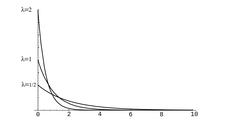
Here [math]\lambda[/math] is any positive constant, depending on the experiment. The reader has seen this density in Example. In Figure we show graphs of several exponential densities for different choices of [math]\lambda[/math].
The exponential density is often used to describe experiments involving a question of the form: How long until something happens? For example, the exponential density is often used to study the time between emissions of particles from a radioactive source.
The cumulative distribution function of the exponential density is easy to
compute. Let [math]T[/math] be an exponentially distributed random variable with parameter
[math]\lambda[/math]. If [math]x \ge 0[/math], then we have
Both the exponential density and the geometric distribution share a property
known as the “memoryless” property. This property was introduced in
Example; it says that
This can be demonstrated to hold for the exponential density by computing both sides of this equation. The right-hand side is just
while the left-hand side is
There is a very important relationship between the exponential density and the Poisson
distribution. We begin by defining [math]X_1,\ X_2,\ \ldots[/math] to be a sequence of
independent exponentially distributed random variables with parameter [math]\lambda[/math]. We
might think of [math]X_i[/math] as denoting the amount of time between the [math]i[/math]th and [math](i+1)[/math]st
emissions of a particle by a radioactive source. (As we shall see in Chapter Expected Value and Variance, we can think of the parameter
[math]\lambda[/math] as representing the reciprocal of the average length of time between
emissions. This parameter is a quantity that might be measured in an actual
experiment of this type.)
We now consider a time interval of length [math]t[/math], and we let [math]Y[/math] denote the random
variable which counts the number of emissions that occur in the time interval. We
would like to calculate the distribution function of
[math]Y[/math] (clearly, [math]Y[/math] is a discrete random variable). If we let [math]S_n[/math] denote the sum
[math]X_1 + X_2 +
\cdots + X_n[/math], then it is easy to see that
Since the event [math]S_{n+1} \le t[/math] is a subset of the event [math]S_n \le t[/math], the above probability is seen to be equal to
We will show in Sums of Independent Random Variables that the density of [math]S_n[/math] is given by the following formula:
This density is an example of a gamma density with parameters [math]\lambda[/math] and [math]n[/math]. The general gamma density allows [math]n[/math] to be any positive real number. We shall not discuss this general density.
It is easy to show by induction on [math]n[/math] that the cumulative distribution function of
[math]S_n[/math] is given by:
Using this expression, the quantity in () is easy to compute; we obtain
which the reader will recognize as the probability that a Poisson-distributed random variable, with parameter [math]\lambda t[/math], takes on the value [math]n[/math].
The above relationship will allow us to simulate a Poisson distribution, once we
have found a way to simulate an exponential density. The following random variable
does the job:
Using Corollary (below), one can derive the above expression (see Exercise). We content ourselves for now with a short calculation that should convince the reader that the random variable [math]Y[/math] has the required property. We have
This last expression is seen to be the cumulative distribution function of an exponentially distributed random variable with parameter [math]\lambda[/math].
To simulate a Poisson random variable [math]W[/math] with parameter [math]\lambda[/math], we simply
generate a sequence of values of an exponentially distributed random variable with
the same parameter, and keep track of the subtotals [math]S_k[/math] of these values. We stop
generating the sequence when the subtotal first exceeds
[math]\lambda[/math]. Assume that we find that
Then the value [math]n[/math] is returned as a simulated value for [math]W[/math].
Example Suppose that customers arrive at random times at a service station with one server, and suppose that each customer is served immediately if no one is ahead of him, but must wait his turn in line otherwise. How long should each customer expect to wait? (We define the waiting time of a customer to be the length of time between the time that he arrives and the time that he begins to be served.)
Let us assume that the interarrival times between successive customers are given by random
variables [math]X_1[/math], [math]X_2[/math], \dots, [math]X_n[/math] that are mutually independent and identically distributed
with an exponential cumulative distribution function given by
Let us assume, too, that the service times for successive customers are given by random variables [math]Y_1[/math], [math]Y_2[/math], \dots, [math]Y_n[/math] that again are mutually independent and identically distributed with another exponential cumulative distribution function given by
The parameters [math]\lambda[/math] and [math]\mu[/math] represent, respectively, the reciprocals of the average time between arrivals of customers and the average service time of the customers. Thus, for example, the larger the value of [math]\lambda[/math], the smaller the average time between arrivals of customers. We can guess that the length of time a customer will spend in the queue depends on the relative sizes of the average interarrival time and the average service time.
It is easy to verify this conjecture by simulation. The program Queue simulates this queueing process. Let [math]N(t)[/math] be the number of customers in the queue at time [math]t[/math]. Then we plot [math]N(t)[/math] as a function of [math]t[/math] for different choices of the parameters [math]\lambda[/math] and [math]\mu[/math] (see Figure).
We note that when [math]\lambda \lt \mu[/math], then [math]1/\lambda \gt 1/\mu[/math], so the average interarrival time is greater than the average service time, i.e., customers are served more quickly, on average, than new ones arrive. Thus, in this case, it is reasonable to expect that [math]N(t)[/math] remains small. However, if [math]\lambda \gt \mu [/math] then customers arrive more quickly than they are served, and, as expected, [math]N(t)[/math] appears to grow without limit.
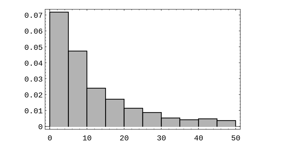
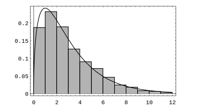
We can now ask: How long will a customer have to wait in the queue for service? To examine this question, we let [math]W_i[/math] be the length of time that the [math]i[/math]th customer has to remain in the system (waiting in line and being served). Then we can present these data in a bar graph, using the program Queue, to give some idea of how the [math]W_i[/math] are distributed (see Figure). (Here [math]\lambda = 1[/math] and [math]\mu = 1.1[/math].)
We see that these waiting times appear to be distributed exponentially. This is always the case when [math]\lambda \lt \mu[/math]. The proof of this fact is too complicated to give here, but we can verify it by simulation for different choices of [math]\lambda[/math] and [math]\mu[/math], as above.
Functions of a Random Variable
Before continuing our list of important densities, we pause to consider random variables which are functions of other random variables. We will prove a general theorem that will allow us to derive expressions such as Equation.
Let [math]X[/math] be a continuous random variable, and suppose that [math]\phi(x)[/math] is a strictly increasing function on the range of [math]X[/math]. Define [math]Y = \phi(X)[/math]. Suppose that [math]X[/math] and [math]Y[/math] have cumulative distribution functions [math]F_X[/math] and [math]F_Y[/math] respectively. Then these functions are related by
Since [math]\phi[/math] is a strictly increasing function on the range of [math]X[/math], the events [math](X \le \phi^{-1}(y))[/math] and [math](\phi(X) \le y)[/math] are equal. Thus, we have
If [math]\phi(x)[/math] is strictly decreasing on the range of [math]X[/math], then we have
Let [math]X[/math] be a continuous random variable, and suppose that [math]\phi(x)[/math] is a strictly increasing function on the range of [math]X[/math]. Define [math]Y = \phi(X)[/math]. Suppose that the density functions of [math]X[/math] and [math]Y[/math] are [math]f_X[/math] and [math]f_Y[/math], respectively. Then these functions are related by
This result follows from Theorem by using the Chain Rule.
If the function [math]\phi[/math] is neither strictly increasing nor strictly decreasing,
then the situation is somewhat more complicated but can be treated by the same
methods. For example, suppose that [math]Y = X^2[/math], Then [math]\phi(x) = x^2[/math], and
Moreover,
We see that in order to express [math]F_Y[/math] in terms of [math]F_X[/math] when [math]Y =
\phi(X)[/math], we have to express [math]P(Y \leq y)[/math] in terms of [math]P(X \leq x)[/math], and this process
will depend in general upon the structure of [math]\phi[/math].
Simulation
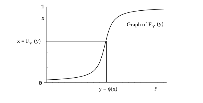
Theorem tells us, among other things, how to simulate on the computer a random variable [math]Y[/math] with a prescribed cumulative distribution function [math]F[/math]. We assume that [math]F(y)[/math] is strictly increasing for those values of [math]y[/math] where [math]0 \lt F(y) \lt 1[/math]. For this purpose, let [math]U[/math] be a random variable which is uniformly distributed on [math][0, 1][/math]. Then [math]U[/math] has cumulative distribution function [math]F_U(u) = u[/math]. Now, if [math]F[/math] is the prescribed cumulative distribution function for [math]Y[/math], then to write [math]Y[/math] in terms of [math]U[/math] we first solve the equation
for [math]y[/math] in terms of [math]u[/math]. We obtain [math]y = F^{-1}(u)[/math]. Note that since [math]F[/math] is an increasing function this equation always has a unique solution (see [[#fig 5.13|Figure]]). Then we set [math]Z = F^{-1}(U)[/math] and obtain, by Theorem,
since [math]F_U(u) = u[/math]. Therefore, [math]Z[/math] and [math]Y[/math] have the same cumulative distribution function. Summarizing, we have the following.
If [math]F(y)[/math] is a given cumulative distribution function that is strictly increasing when [math]0 \lt F(y) \lt 1[/math] and if [math]U[/math] is a random variable with uniform distribution on [math][0,1][/math], then
has the cumulative distribution [math]F(y)[/math].
Thus, to simulate a random variable with a given cumulative distribution [math]F[/math] we need only set [math]Y = F^{-1}(\mbox{rnd})[/math].
Normal Density
We now come to the most important density function, the normal density function. We have seen in Chapter Combinatorics that the binomial distribution functions are bell-shaped, even for moderate size values of [math]n[/math]. We recall that a binomially-distributed random variable with parameters [math]n[/math] and [math]p[/math] can be considered to be the sum of [math]n[/math] mutually independent 0-1 random variables. A very important theorem in probability theory, called the Central Limit Theorem, states that under very general conditions, if we sum a large number of mutually independent random variables, then the distribution of the sum can be closely approximated by a certain specific continuous density, called the normal density. This theorem will be discussed in Central Limit Theorem.
The normal density function with parameters [math]\mu[/math] and [math]\sigma[/math] is defined as follows:
The parameter [math]\mu[/math] represents the “center” of the density (and in Chapter \ref{chp 6}, we will show that it is the average, or expected, value of the density). The parameter [math]\sigma[/math] is a measure of the “spread” of the density, and thus it is assumed to be positive. (In Chapter \ref{chp 6}, we will show that [math]\sigma[/math] is the standard deviation of the density.) We note that it is not at all obvious that the above function is a density, i.e., that its integral over the real line equals 1. The cumulative distribution function is given by the formula
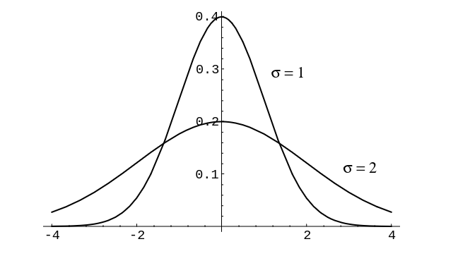
In Figure we have included for comparison a plot of the normal density for the cases [math]\mu = 0[/math] and [math]\sigma = 1[/math], and [math]\mu = 0[/math] and [math]\sigma = 2[/math].
One cannot write [math]F_X[/math] in terms of simple functions. This leads to several
problems. First of all, values of [math]F_X[/math] must be computed using numerical
integration. Extensive tables exist containing values of this function (see Appendix A).
Secondly, we cannot write [math]F^{-1}_X[/math] in closed form, so we cannot use Corollary to help
us simulate a normal random variable. For this reason, special methods have been developed for
simulating a normal distribution. One such method relies on the fact that if [math]U[/math] and [math]V[/math] are
independent random variables with uniform densities on
[math][0,1][/math], then the random variables
and
are independent, and have normal density functions with parameters [math]\mu = 0[/math] and [math]\sigma = 1[/math]. (This is not obvious, nor shall we prove it here. See Box and Muller.[Notes 1])
Let [math]Z[/math] be a normal random variable with parameters [math]\mu = 0[/math] and [math]\sigma = 1[/math]. A
normal random variable with these parameters is said to be a standard normal
random variable. It is an important and useful
fact that if we write
then [math]X[/math] is a normal random variable with parameters [math]\mu[/math] and [math]\sigma[/math]. To show this, we will use Theorem. We have [math]\phi(z) = \sigma z + \mu[/math], [math]\phi^{-1}(x) = (x - \mu)/\sigma[/math], and
The reader will note that this last expression is the density function with parameters [math]\mu[/math] and [math]\sigma[/math], as claimed.
We have seen above that it is possible to simulate a standard normal random variable [math]Z[/math].
If we wish to simulate a normal random variable [math]X[/math] with parameters [math]\mu[/math] and [math]\sigma[/math],
then we need only transform the simulated values for [math]Z[/math] using the equation [math]X = \sigma Z +
\mu[/math].
Suppose that we wish to calculate the value of a cumulative distribution function for the normal random
variable [math]X[/math], with parameters [math]\mu[/math] and [math]\sigma[/math]. We can reduce this calculation to one
concerning the standard normal random variable [math]Z[/math] as follows:
This last expression can be found in a table of values of the cumulative distribution function for a standard normal random variable. Thus, we see that it is unnecessary to make tables of normal distribution functions with arbitrary [math]\mu[/math] and [math]\sigma[/math].
The process of changing a normal random variable to a standard normal random variable is
known as standardization. If [math]X[/math] has a normal distribution with parameters [math]\mu[/math] and
[math]\sigma[/math] and if
then [math]Z[/math] is said to be the standardized version of [math]X[/math].
The following example shows how we use the standardized version of a normal random variable [math]X[/math] to compute specific probabilities relating to [math]X[/math].
Example Suppose that [math]X[/math] is a normally distributed random variable with parameters [math]\mu = 10[/math] and [math]\sigma = 3[/math]. Find the probability that [math]X[/math] is between 4 and 16.
To solve this problem, we note that [math]Z = (X-10)/3[/math] is the standardized version of [math]X[/math].
So, we have
This last expression can be evaluated by using tabulated values of the standard normal distribution function (see \ref{app_a}); when we use this table, we find that [math]F_Z(2) = .9772[/math] and [math]F_Z(-2) = .0228[/math]. Thus, the answer is .9544.
In Chapter Expected Value and Variance, we will see that the parameter [math]\mu[/math] is the mean, or average value, of the random variable [math]X[/math]. The parameter [math]\sigma[/math] is a measure of the spread of the random variable, and is called the standard deviation. Thus, the question asked in this example is of a typical type, namely, what is the probability that a random variable has a value within two standard deviations of its average value.
Maxwell and Rayleigh Densities
Example Suppose that we drop a dart on a large table top, which we consider as the [math]xy[/math]-plane, and suppose that the [math]x[/math] and [math]y[/math] coordinates of the dart point are independent and have a normal distribution with parameters [math]\mu = 0[/math] and [math]\sigma = 1[/math]. How is the distance of the point from the origin distributed?
This problem arises in physics when it is assumed that a moving particle in [math]R^n[/math] has components of the velocity that are mutually independent and normally distributed and it is desired to find the density of the speed of the particle. The density in the case [math]n = 3[/math] is called the Maxwell density.
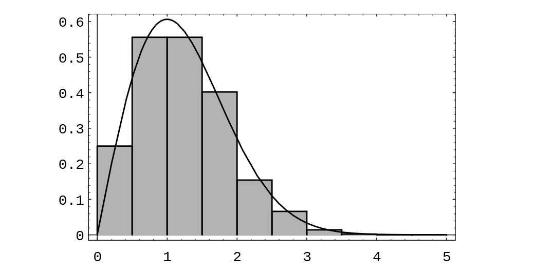
The density in the case [math]n = 2[/math] (i.e. the dart board experiment described above) is called the Rayleigh density. We can simulate this case by picking independently a pair of coordinates [math](x,y)[/math], each from a normal distribution with [math]\mu = 0[/math] and [math]\sigma = 1[/math] on [math](-\infty,\infty)[/math], calculating the distance [math]r = \sqrt{x^2 + y^2}[/math] of the point [math](x,y)[/math] from the origin, repeating this process a large number of times, and then presenting the results in a bar graph. The results are shown in Figure.
We have also plotted the theoretical density
This will be derived in Sums of Independent Random Variables; see Example.
Chi-Squared Density
We return to the problem of independence of traits discussed in Example. It is frequently the case that we have two traits, each of which have several different values. As was seen in the example, quite a lot of calculation was needed even in the case of two values for each trait. We now give another method for testing independence of traits, which involves much less calculation. Example Suppose that we have the data shown in Table concerning grades and gender of students in a Calculus class.
| Female | Male | ||
| A | 37 | 56 | 93 |
| B | 63 | 60 | 123 |
| C | 47 | 43 | 90 |
| Below C | 5 | 8 | 13 |
| 152 | 167 | 319 |
We can use the same sort of model in this situation as was used in Example \ref{exam 5.6}. We imagine that we have an urn with 319 balls of two colors, say blue and red, corresponding to females and males, respectively. We now draw 93 balls, without replacement, from the urn. These balls correspond to the grade of A. We continue by drawing 123 balls, which correspond to the grade of B. When we finish, we have four sets of balls, with each ball belonging to exactly one set. (We could have stipulated that the balls were of four colors, corresponding to the four possible grades. In this case, we would draw a subset of size 152, which would correspond to the females. The balls remaining in the urn would correspond to the males. The choice does not affect the final determination of whether we should reject the hypothesis of independence of traits.)
The expected data set can be determined in exactly the same way as in Example. If we do this, we obtain the expected values shown in Table.
| Female | Male | ||
| A | 44.3 | 48.7 | 93 |
| B | 58.6 | 64.4 | 123 |
| C | 42.9 | 47.1 | 90 |
| Below C | 6.2 | 6.8 | 13 |
| 152 | 167 | 319 |
Even if the traits are independent, we would still expect to see some differences between the numbers in corresponding boxes in the two tables. However, if the differences are large, then we might suspect that the two traits are not independent. In Example, we used the probability distribution of the various possible data sets to compute the probability of finding a data set that differs from the expected data set by at least as much as the actual data set does. We could do the same in this case, but the amount of computation is enormous.
Instead, we will describe a single number which does a good job of measuring how far a given data set is from the expected one. To quantify how far apart the two sets of numbers are, we could sum the squares of the differences of the corresponding numbers. (We could also sum the absolute values of the differences, but we would not want to sum the differences.) Suppose that we have data in which we expect to see 10 objects of a certain type, but instead we see 18, while in another case we expect to see 50 objects of a certain type, but instead we see 58. Even though the two differences are about the same, the first difference is more surprising than the second, since the expected number of outcomes in the second case is quite a bit larger than the expected number in the first case. One way to correct for this is to divide the individual squares of the differences by the expected number for that box. Thus, if we label the values in the eight boxes in the first table by [math]O_i[/math] (for observed values) and the values in the eight boxes in the second table by [math]E_i[/math] (for expected values), then the following expression might be a reasonable one to use to measure how far the observed data is from what is expected:
This expression is a random variable, which is usually denoted by the symbol $\chi^2$, pronounced “ki-squared.” It is called this because, under the assumption of independence of the two traits, the density of this random variable can be computed and is approximately equal to a density called the chi-squared density. We choose not to give the explicit expression for this density, since it involves the gamma function, which we have not discussed. The chi-squared density is, in fact, a special case of the general gamma density.
In applying the chi-squared density, tables of values of this density are used, as in
the case of the normal density. The chi-squared density has one parameter [math]n[/math], which
is called the number of degrees of freedom. The number [math]n[/math] is
usually easy to determine from the problem at hand. For example, if we are checking
two traits for independence, and the two traits have [math]a[/math] and [math]b[/math] values, respectively,
then the number of degrees of freedom of the random variable [math]\chi^2[/math] is
[math](a-1)(b-1)[/math]. So, in the example at hand, the number of degrees of freedom is 3.
We recall that in this example, we are trying to test for independence of the two traits of
gender and grades. If we assume these traits are independent, then the ball-and-urn model
given above gives us a way to simulate the experiment. Using a computer, we have performed
1000 experiments, and for each one, we have calculated a value of the random variable
[math]\chi^2[/math]. The results are shown in Figure, together with the
chi-squared density function with three degrees of freedom.
As we stated above, if the value of the random variable [math]\chi^2[/math] is large, then we
would tend not to believe that the two traits are independent. But how large is
large? The actual value of this random variable for the data above is 4.13. In
Figure, we have shown the chi-squared density with 3 degrees of freedom.
It can be seen that the value 4.13 is larger than most of the values taken on by this
random variable.
Typically, a statistician will compute the value [math]v[/math] of the random variable [math]\chi^2[/math], just as we have done. Then, by looking in a table of values of the chi-squared density, a value [math]v_0[/math] is determined which is only exceeded 5% of the time. If [math]v \ge v_0[/math], the statistician rejects the hypothesis that the two traits are independent. In the present case, [math]v_0 = 7.815[/math], so we would not reject the hypothesis that the two traits are independent.
Cauchy Density
The following example is from Feller.[Notes 2]
Example Suppose that a mirror is mounted on a vertical axis, and is free to revolve about that axis. The axis of the mirror is 1 foot from a straight wall of infinite length. A pulse of light is shown onto the mirror, and the reflected ray hits the wall. Let [math]\phi[/math] be the angle between the reflected ray and the line that is perpendicular to the wall and that runs through the axis of the mirror. We assume that [math]\phi[/math] is uniformly distributed between [math]-\pi/2[/math] and [math]\pi/2[/math]. Let [math]X[/math] represent the distance between the point on the wall that is hit by the reflected ray and the point on the wall that is closest to the axis of the mirror. We now determine the density of [math]X[/math].
Let [math]B[/math] be a fixed positive quantity. Then [math]X \ge B[/math] if and only if [math]\tan(\phi) \ge
B[/math], which happens if and only if [math]\phi \ge \arctan(B)[/math]. This happens with
probability
Thus, for positive [math]B[/math], the cumulative distribution function of [math]X[/math] is
Therefore, the density function for positive [math]B[/math] is
Since the physical situation is symmetric with respect to [math]\phi = 0[/math], it is easy to see that the above expression for the density is correct for negative values of [math]B[/math] as well.
The Law of Large Numbers, which we will discuss in Chapter Law of Large Numbers, states that in many cases, if we take the average of independent values of a random variable, then the average approaches a specific number as the number of values increases. It turns out that if one does this with a Cauchy-distributed random variable, the average does not approach any specific number.
General references
Doyle, Peter G. (2006). "Grinstead and Snell's Introduction to Probability" (PDF). Retrieved June 6, 2024.
