guide:A070937c41: Difference between revisions
mNo edit summary |
mNo edit summary |
||
| Line 27: | Line 27: | ||
not 1, as it should be. | not 1, as it should be. | ||
<div id="fig 2.05" class="d-flex justify-content-center"> | <div id="fig 2.05" class="d-flex justify-content-center"> | ||
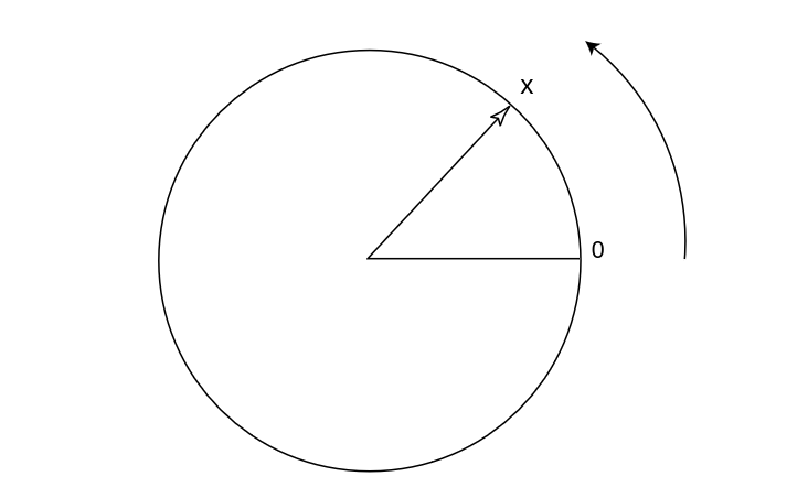
[[File:guide_e6d15_PSfig2-12arc.png | | [[File:guide_e6d15_PSfig2-12arc.png | 500px | thumb | A spinner. ]] | ||
</div> | </div> | ||
| Line 78: | Line 78: | ||
[[#fig 2.4|Figure]]). | [[#fig 2.4|Figure]]). | ||
<div id="fig 2.3" class="d-flex justify-content-center"> | <div id="fig 2.3" class="d-flex justify-content-center"> | ||
[[File:guide_e6d15_PSfig2-3.png | | [[File:guide_e6d15_PSfig2-3.png | 500px | thumb | Area under <math>y = x^2.</math> ]] | ||
</div> | </div> | ||
From these experiments we would estimate the area to be about 1/3. Of course, | From these experiments we would estimate the area to be about 1/3. Of course, | ||
| Line 92: | Line 92: | ||
did achieve this accuracy. | did achieve this accuracy. | ||
<div id="fig 2.4" class="d-flex justify-content-center"> | <div id="fig 2.4" class="d-flex justify-content-center"> | ||
[[File:guide_e6d15_PSfig2-4.png | | [[File:guide_e6d15_PSfig2-4.png | 500px | thumb | Computing the area by simulation. ]] | ||
</div> | </div> | ||
This same argument works for any region <math>E</math> of the unit square. For example, | This same argument works for any region <math>E</math> of the unit square. For example, | ||
| Line 133: | Line 133: | ||
<div id="fig 2.6" class="d-flex justify-content-center"> | <div id="fig 2.6" class="d-flex justify-content-center"> | ||
[[File:guide_e6d15_PSfig2-6.png | | [[File:guide_e6d15_PSfig2-6.png | 500px | thumb |Buffon's experiment.]] | ||
</div> | </div> | ||
Now we assume that when the needle drops, the pair <math>(\theta,d)</math> is chosen at | Now we assume that when the needle drops, the pair <math>(\theta,d)</math> is chosen at | ||
| Line 152: | Line 152: | ||
<div id="fig 2.7" class="d-flex justify-content-center"> | <div id="fig 2.7" class="d-flex justify-content-center"> | ||
[[File:guide_e6d15_PSfig2-7.png | | [[File:guide_e6d15_PSfig2-7.png | 500px | thumb |Set <math>E</math> of pairs <math>(\theta, d)</math> with <math>d < {\frac{1}{2}} \sin \theta</math>. ]] | ||
</div>} \sin \theta</math>.}{fig 2.7} | </div>} \sin \theta</math>.}{fig 2.7} | ||
The program ''' BuffonsNeedle''' simulates this experiment. In | The program ''' BuffonsNeedle''' simulates this experiment. In | ||
| Line 170: | Line 170: | ||
<div id="fig 2.8" class="d-flex justify-content-center"> | <div id="fig 2.8" class="d-flex justify-content-center"> | ||
[[File:guide_e6d15_PSfig2-8.png | | [[File:guide_e6d15_PSfig2-8.png | 500px | thumb | Simulation of Buffon's needle experiment. ]] | ||
</div> | </div> | ||
In each of our examples so far, events of the same size are equally likely. | In each of our examples so far, events of the same size are equally likely. | ||
| Line 208: | Line 208: | ||
\linebreak[4]<math>f(x)</math>. | \linebreak[4]<math>f(x)</math>. | ||
<div id="fig 2.8.5" class="d-flex justify-content-center"> | <div id="fig 2.8.5" class="d-flex justify-content-center"> | ||
[[File:guide_e6d15_PSfig2-8-5.png | | [[File:guide_e6d15_PSfig2-8-5.png | 500px | thumb | Sum of two random numbers. ]] | ||
</div> | </div> | ||
| Line 221: | Line 221: | ||
<div id="fig 2.8.6" class="d-flex justify-content-center"> | <div id="fig 2.8.6" class="d-flex justify-content-center"> | ||
[[File:guide_e6d15_PSfig2-8-6.png | | [[File:guide_e6d15_PSfig2-8-6.png | 500px | thumb | Sum of 100 random numbers. ]] | ||
</div> | </div> | ||
| Line 256: | Line 256: | ||
simulation, it is convenient to include certain simplifications, which we describe in turn: | simulation, it is convenient to include certain simplifications, which we describe in turn: | ||
<div id="fig 2.10" class="d-flex justify-content-center"> | <div id="fig 2.10" class="d-flex justify-content-center"> | ||
[[File:guide_e6d15_PSfig2-10.png | | [[File:guide_e6d15_PSfig2-10.png | 500px | thumb |Random chord. ]] | ||
</div> | </div> | ||
<ul><li> To simulate this case, we choose values for <math>x</math> and <math>y</math> from <math>[-1,1]</math> at | <ul><li> To simulate this case, we choose values for <math>x</math> and <math>y</math> from <math>[-1,1]</math> at | ||
| Line 298: | Line 298: | ||
of every 100th trial up to 10,00 trials. | of every 100th trial up to 10,00 trials. | ||
<div id="fig 2.11" class="d-flex justify-content-center"> | <div id="fig 2.11" class="d-flex justify-content-center"> | ||
[[File:guide_e6d15_PSfig2-11.png | | [[File:guide_e6d15_PSfig2-11.png | 500px | thumb | Bertrand's paradox. ]] | ||
</div> | </div> | ||
It is interesting to observe that these fractions are ''not'' the same in | It is interesting to observe that these fractions are ''not'' the same in | ||
Revision as of 01:00, 10 June 2024
In this section we shall show how we can use computer simulations for experiments that have a whole continuum of possible outcomes.
Probabilities
Example We begin by constructing a spinner, which consists of a circle of unit circumference and a pointer as shown in Figure. We pick a point on the circle and label it 0, and then label every other point on the circle with the distance, say [math]x[/math], from 0 to that point, measured counterclockwise. The experiment consists of spinning the pointer and recording the label of the point at the tip of the pointer. We let the random variable [math]X[/math] denote the value of this outcome. The sample space is clearly the interval [math][0, 1)[/math]. We would like to construct a probability model in which each outcome is equally likely to occur.
If we proceed as we did in Chapter Discrete Probability Distributions for experiments with a finite number of possible outcomes, then we must assign the probability 0 to each outcome, since otherwise, the sum of the probabilities, over all of the possible outcomes, would not equal 1. (In fact, summing an uncountable number of real numbers is a tricky business; in particular, in order for such a sum to have any meaning, at most countably many of the summands can be different than 0.) However, if all of the assigned probabilities are 0, then the sum is 0, not 1, as it should be.
In the next section, we will show how to construct a probability model in this situation.
At present, we will assume that such a model can be constructed. We will also assume that
in this model, if [math]E[/math] is an arc of the circle, and [math]E[/math] is of length [math]p[/math], then the model
will assign the probability [math]p[/math] to [math]E[/math]. This means that if the pointer is spun, the
probability that it ends up pointing to a point in [math]E[/math] equals [math]p[/math], which is certainly a
reasonable thing to expect.
To simulate this experiment on a computer is an easy matter. Many computer software
packages have a function which returns a random real number in the interval [math][0, 1][/math].
Actually, the returned value is always a rational number, and the values are determined by
an algorithm, so a sequence of such values is not truly random. Nevertheless,
the sequences produced by such algorithms behave much like theoretically random sequences,
so we can use such sequences in the simulation of experiments. On occasion, we will need
to refer to such a function. We will call this function [math]rnd[/math].
Monte Carlo Procedure and Areas
It is sometimes desirable to estimate quantities whose exact values are difficult or impossible to calculate exactly. In some of these cases, a procedure involving chance, called a Monte Carlo procedure, can be used to provide such an estimate. Example In this example we show how simulation can be used to estimate areas of plane figures. Suppose that we program our computer to provide a pair [math](x,y)[/math] or numbers, each chosen independently at random from the interval [math][0,1][/math]. Then we can interpret this pair [math](x,y)[/math] as the coordinates of a point chosen at random from the unit square. Events are subsets of the unit square. Our experience with Example suggests that the point is equally likely to fall in subsets of equal area. Since the total area of the square is 1, the probability of the point falling in a specific subset [math]E[/math] of the unit square should be equal to its area. Thus, we can estimate the area of any subset of the unit square by estimating the probability that a point chosen at random from this square falls in the subset.
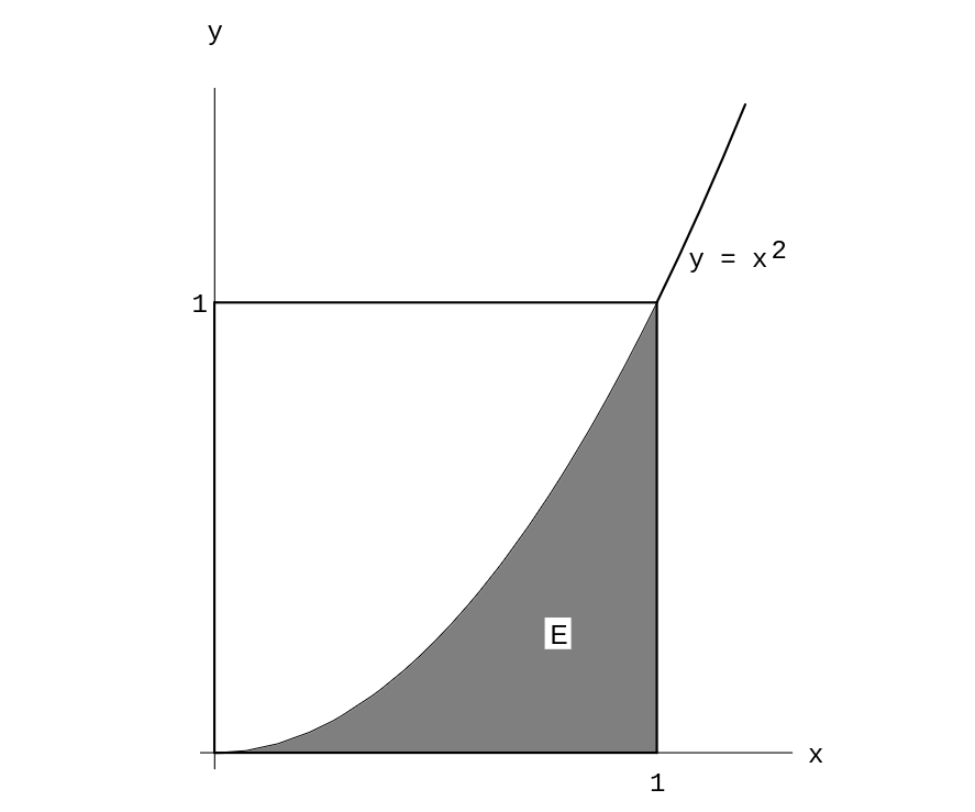
We can use this method to estimate the area of the region [math]E[/math] under the curve
[math]y = x^2[/math] in the unit square (see Figure). We choose a large number of
points [math](x,y)[/math] at random and record what fraction of them fall in the region [math]E
= \{\,(x,y):y \leq x^2\,\}[/math].
The program MonteCarlo will carry out this experiment for us.
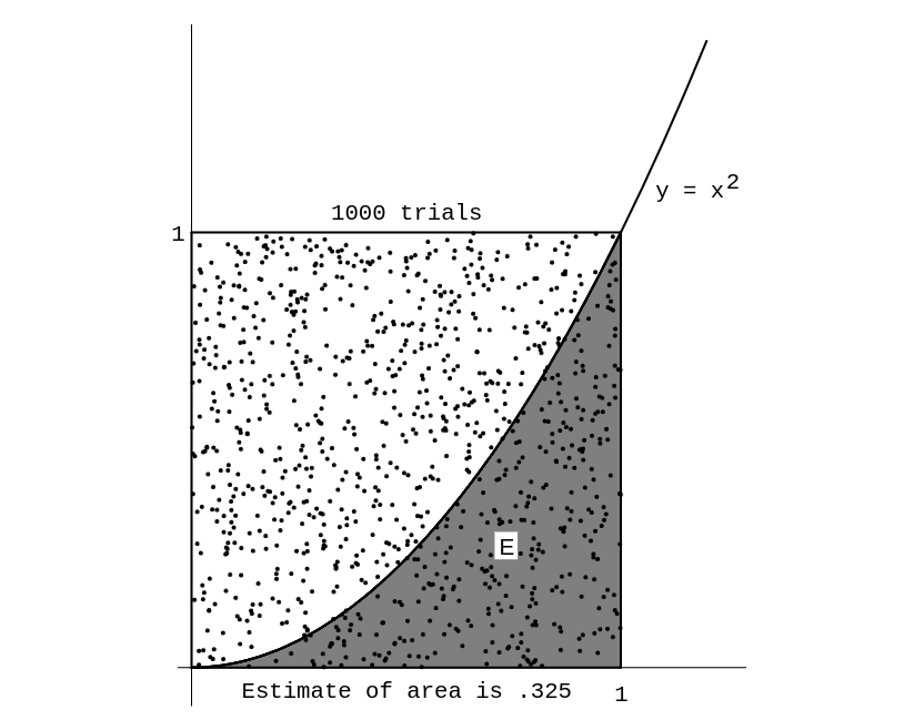
Running this program for 10,00 experiments gives an estimate of .325 (see
Figure).
From these experiments we would estimate the area to be about 1/3. Of course, for this simple region we can find the exact area by calculus. In fact,
We have remarked in Chapter \ref{chp 1} that, when we simulate an experiment of this type [math]n[/math] times to estimate a probability, we can expect the answer to be in error by at most [math]1/\sqrt n[/math] at least 95 percent of the time. For 10,00 experiments we can expect an accuracy of 0.01, and our simulation did achieve this accuracy.
This same argument works for any region [math]E[/math] of the unit square. For example, suppose [math]E[/math] is the circle with center [math](1/2,1/2)[/math] and radius 1/2. Then the probability that our random point [math](x,y)[/math] lies inside the circle is equal to the area of the circle, that is,
If we did not know the value of [math]\pi[/math], we could estimate the value by performing this experiment a large number of times!
The above example is not the only way of estimating the value of [math]\pi[/math] by a chance experiment. Here is another way, discovered by Buffon.[Notes 1]
Buffon's Needle
Example Suppose that we take a card table and draw across the top surface a set of parallel lines a unit distance apart. We then drop a common needle of unit length at random on this surface and observe whether or not the needle lies across one of the lines. We can describe the possible outcomes of this experiment by coordinates as follows: Let [math]d[/math] be the distance from the center of the needle to the nearest line. Next, let [math]L[/math] be the line determined by the needle, and define [math]\theta[/math] as the acute angle that the line [math]L[/math] makes with the set of parallel lines. (The reader should certainly be wary of this description of the sample space. We are attempting to coordinatize a set of line segments. To see why one must be careful in the choice of coordinates, see Example \ref {exam 2.1.5}.) Using this description, we have [math]0 \leq d \leq 1/2[/math], and [math]0 \leq \theta \leq \pi/2[/math]. Moreover, we see that the needle lies across the nearest line if and only if the hypotenuse of the triangle (see Figure \ref{fig 2.6}) is less than half the length of the needle, that is,
Now we assume that when the needle drops, the pair [math](\theta,d)[/math] is chosen at random from the rectangle [math]0 \leq \theta \leq \pi/2[/math], [math]0 \leq d \leq 1/2[/math]. We observe whether the needle lies across the nearest line (i.e., whether [math]d \leq (1/2)\sin\theta[/math]). The probability of this event [math]E[/math] is the fraction of the area of the rectangle which lies inside [math]E[/math] (see Figure). Now the area of the rectangle is [math]\pi/4[/math], while the area of [math]E[/math] is
Hence, we get
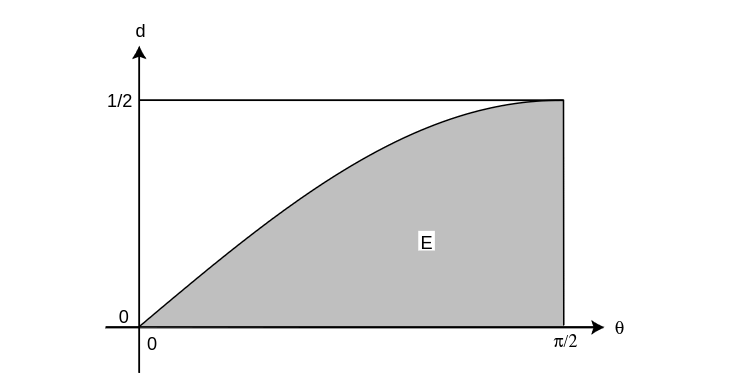
} \sin \theta</math>.}{fig 2.7}
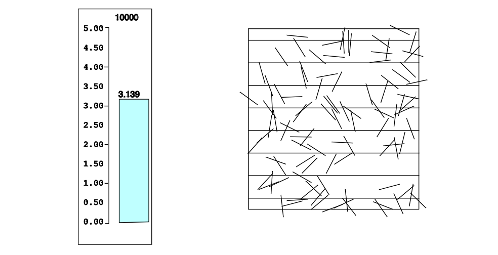
The program BuffonsNeedle simulates this experiment. In Figure, we show the position of every 100th needle in a run of the program in which 10,00 needles were “dropped.” Our final estimate for [math]\pi[/math] is 3.139. While this was within 0.003 of the true value for [math]\pi[/math] we had no right to expect such accuracy. The reason for this is that our simulation estimates [math]P(E)[/math]. While we can expect this estimate to be in error by at most 0.001, a small error in [math]P(E)[/math] gets magnified when we use this to compute [math]\pi = 2/P(E)[/math]. Perlman and Wichura, in their article “Sharpening Buffon's Needle,”[Notes 2] show that we can expect to have an error of not more than [math]5/\sqrt n[/math] about 95 percent of the time. Here [math]n[/math] is the number of needles dropped. Thus for 10,00 needles we should expect an error of no more than 0.05, and that was the case here. We see that a large number of experiments is necessary to get a decent estimate for [math]\pi[/math].
In each of our examples so far, events of the same size are equally likely. Here is an example where they are not. We will see many other such examples later.
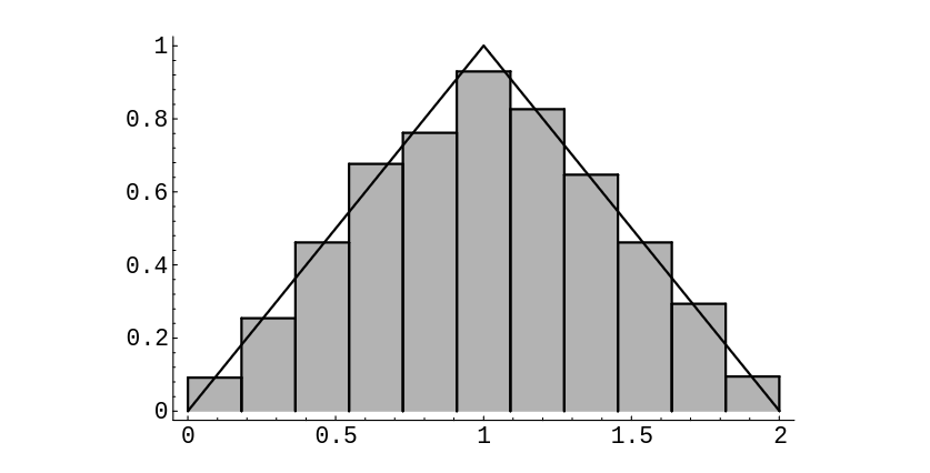
Example Suppose that we choose two random real numbers in [math][0,1][/math] and add them together. Let [math]X[/math] be the sum. How is [math]X[/math] distributed?
To help understand the answer to this question, we can use the program
Areabargraph. This program produces a bar graph with the
property that on each interval, the area, rather than the height, of the bar is equal to
the fraction of outcomes that fell in the corresponding interval. We have carried out this
experiment 1000 times; the data is shown in Figure. It appears that the
function defined by
fits the data very well. (It is shown in the figure.) In the next section, we will see that this function is the “right” function. By this we mean that if [math]a[/math] and [math]b[/math] are any two real numbers between [math]0[/math] and [math]2[/math], with [math]a \le b[/math], then we can use this function to calculate the probability that [math]a \le X \le b[/math]. To understand how this calculation might be performed, we again consider Figure. Because of the way the bars were constructed, the sum of the areas of the bars corresponding to the interval [math][a, b][/math] approximates the probability that [math]a \le X \le b[/math]. But the sum of the areas of these bars also approximates the integral
This suggests that for an experiment with a continuum of possible outcomes, if we find a function with the above property, then we will be able to use it to calculate probabilities. In the next section, we will show how to determine the function \linebreak[4][math]f(x)[/math].
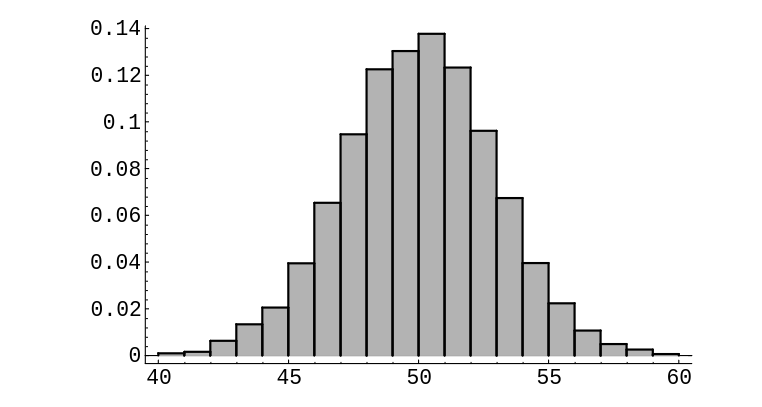
Example Suppose that we choose 100 random numbers in [math][0, 1][/math], and let [math]X[/math] represent their sum. How is [math]X[/math] distributed? We have carried out this experiment 10000 times; the results are shown in Figure. It is not so clear what function fits the bars in this case. It turns out that the type of function which does the job is called a normal density function. This type of function is sometimes referred to as a “bell-shaped” curve. It is among the most important functions in the subject of probability, and will be formally defined in Section of Chapter Distributions and Densities.
Our last example explores the fundamental question of how probabilities are
assigned.
Bertrand's Paradox
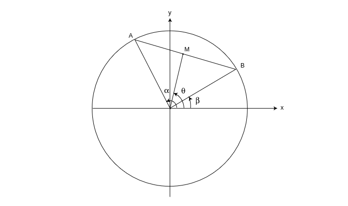
Example A chord of a circle is a line segment both of whose endpoints lie on the circle. Suppose that a chord is drawn at random in a unit circle. What is the probability that its length exceeds [math]\sqrt 3[/math]? Our answer will depend on what we mean by random, which will depend, in turn, on what we choose for coordinates. The sample space [math]\Omega[/math] is the set of all possible chords in the circle. To find coordinates for these chords, we first introduce a rectangular coordinate system with origin at the center of the circle (see Figure). We note that a chord of a circle is perpendicular to the radial line containing the midpoint of the chord. We can describe each chord by giving:
- The rectangular coordinates [math](x,y)[/math] of the midpoint [math]M[/math], or
- The polar coordinates [math](r,\theta)[/math] of the midpoint [math]M[/math], or
- The polar coordinates [math](1,\alpha)[/math] and [math](1,\beta)[/math] of the endpoints [math]A[/math] and [math]B[/math].
In each case we shall interpret at random to mean: choose these coordinates at random. We can easily estimate this probability by computer simulation. In programming this simulation, it is convenient to include certain simplifications, which we describe in turn:
- To simulate this case, we choose values for [math]x[/math] and [math]y[/math] from [math][-1,1][/math] at
random. Then we check whether [math]x^2 + y^2 \leq 1[/math]. If not, the point [math]M =
(x,y)[/math] lies outside the circle and cannot be the midpoint of any chord, and we
ignore it. Otherwise, [math]M[/math] lies inside the circle and is the midpoint of a
unique chord, whose length [math]L[/math] is given by the formula:
[[math]] L = 2\sqrt{1 - (x^2 + y^2)}\ . [[/math]]
- To simulate this case, we take account of the fact that any rotation of
the circle does not change the length of the chord, so we might as well assume
in advance that the chord is horizontal. Then we
choose [math]r[/math] from [math][-1,1][/math] at random, and compute the length of the resulting
chord with midpoint [math](r,\pi/2)[/math] by the formula:
[[math]] L = 2\sqrt{1 - r^2}\ . [[/math]]
- To simulate this case, we assume that one endpoint, say [math]B[/math], lies at
[math](1, 0)[/math] (i.e., that [math]\beta = 0[/math]). Then we choose a value for [math]\alpha[/math] from
[math][0,2\pi][/math] at random and compute the length of the resulting chord, using the
Law of Cosines, by the formula:
[[math]] L = \sqrt{2 - 2\cos\alpha}\ . [[/math]]
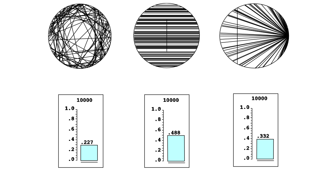
The program BertrandsParadox carries out this simulation. Running this program produces the results shown in Figure. In the first circle in this figure, a smaller circle has been drawn. Those chords which intersect this smaller circle have length at least [math]\sqrt 3[/math]. In the second circle in the figure, the vertical line intersects all chords of length at least [math]\sqrt 3[/math]. In the third circle, again the vertical line intersects all chords of length at least [math]\sqrt 3[/math]. In each case we run the experiment a large number of times and record the fraction of these lengths that exceed [math]\sqrt 3[/math]. We have printed the results of every 100th trial up to 10,00 trials.
It is interesting to observe that these fractions are not the same in the three cases; they depend on our choice of coordinates. This phenomenon was first observed by Bertrand, and is now known as Bertrand's paradox.[Notes 3] It is actually not a paradox at all; it is merely a reflection of the fact that different choices of coordinates will lead to different assignments of probabilities. Which assignment is “correct” depends on what application or interpretation of the model one has in mind.
One can imagine a real experiment involving throwing long straws at a circle
drawn on a card table. A “correct” assignment of coordinates should not depend on
where the circle lies on the card table, or where the card table sits in the room.
Jaynes[Notes 4] has shown that the only assignment which
meets this requirement is (2). In this sense, the assignment (2) is the natural, or
“correct” one (see Exercise \ref{exer2.1.11}).
We can easily see in each case what the true probabilities are if we note that
[math]\sqrt 3[/math] is the length of the side of an inscribed equilateral triangle.
Hence, a chord has length [math]L \gt \sqrt 3[/math] if its midpoint has distance [math]d \lt 1/2[/math]
from the origin (see Figure). The following calculations determine
the probability that [math]L \gt \sqrt 3[/math] in each of the three cases.
- [math]L \gt \sqrt 3[/math] if[math](x,y)[/math] lies inside a circle of radius 1/2, which occurs with
probability
[[math]] p = \frac{\pi(1/2)^2}{\pi(1)^2} = \frac14\ . [[/math]]
- [math]L \gt \sqrt 3[/math] if [math]|r| \lt 1/2[/math], which occurs with probability
[[math]] \frac{1/2 - (-1/2)}{1 - (-1)} = \frac12\ . [[/math]]
- [math]L \gt \sqrt 3[/math] if [math]2\pi/3 \lt \alpha \lt 4\pi/3[/math], which occurs with probability
[[math]] \frac{4\pi/3 - 2\pi/3}{2\pi - 0} = \frac13\ . [[/math]]
We see that our simulations agree quite well with these theoretical values.
Historical Remarks
G. L. Buffon (1707--1788) was a natural scientist in the eighteenth century who applied probability to a number of his investigations. His work is found in his monumental 44-volume Histoire Naturelle and its supplements.[Notes 5] For example, he presented a number of mortality tables and used them to compute, for each age group, the expected remaining lifetime. From his table he observed: the expected remaining lifetime of an infant of one year is 33 years, while that of a man of 21 years is also approximately 33 years. Thus, a father who is not yet 21 can hope to live longer than his one year old son, but if the father is 40, the odds are already 3 to 2 that his son will outlive him.[Notes 6]
Buffon wanted to show that not all probability calculations rely only on
algebra, but that some rely on geometrical calculations. One such problem
was his famous “needle problem” as discussed in this
chapter.[Notes 7] In his original formulation, Buffon describes a game
in which two gamblers drop a loaf of French bread on a wide-board floor and bet on
whether or not the loaf falls across a crack in the floor. Buffon asked: what
length [math]L[/math] should the bread loaf be, relative to the width [math]W[/math] of the
floorboards, so that the game is fair. He found the correct answer ([math]L =
(\pi/4)W[/math]) using essentially the methods described in this chapter. He also
considered the case of a checkerboard floor, but gave the wrong answer in this
case. The correct answer was given later by Laplace.
The literature contains descriptions of a number of experiments that were
actually carried out to estimate [math]\pi[/math] by this method of dropping needles.
N. T. Gridgeman[Notes 8] discusses the experiments shown in Table.
| Experimenter | Length of needle | Number of casts | Number of crossings | Estimate for [math]\pi[/math] |
|---|---|---|---|---|
| Wolf, 1850 | .8 | 5000 | 2532 | 3.1596 |
| Smith, 1855 | .6 | 3204 | 1218.5 | 3.1553 |
| De Morgan, c.1860 | 1.0 | 600 | 382.5 | 3.137 |
| Fox, 1864 | .75 | 1030 | 489 | 3.1595 |
| Lazzerini, 1901 | .83 | 3408 | 1808 | 3.1415929 |
| Reina, 1925 | .5419 | 2520 | 869 | 3.1795 |
(The halves for the number of crossing comes from a compromise when it could not be decided if a crossing had actually occurred.) He observes, as we have, that 10,00 casts could do no more than establish the first decimal place of [math]\pi[/math] with reasonable confidence. Gridgeman points out that, although none of the experiments used even 10,00 casts, they are surprisingly good, and in some cases, too good. The fact that the number of casts is not always a round number would suggest that the authors might have resorted to clever stopping to get a good answer. Gridgeman comments that Lazzerini's estimate turned out to agree with a well-known approximation to [math]\pi[/math], [math]355/113 = 3.1415929[/math], discovered by the fifth-century Chinese mathematician, Tsu Ch'ungchih. Gridgeman says that he did not have Lazzerini's original report, and while waiting for it (knowing only the needle crossed a line 1808 times in 3408 casts) deduced that the length of the needle must have been 5/6. He calculated this from Buffon's formula, assuming [math]\pi = 355/113[/math]:
Even with careful planning one would have to be extremely lucky to be able to stop so cleverly.
The second author likes to trace his interest in probability theory to the Chicago
World's Fair of 1933 where he observed a mechanical device dropping
needles and displaying the ever-changing estimates for the value of [math]\pi[/math]. (The first author
likes to trace his interest in probability theory to the second author.)
General references
Doyle, Peter G. (2006). "Grinstead and Snell's Introduction to Probability" (PDF). Retrieved June 6, 2024.
Notes
- G. L. Buffon, in “Essai d'Arithmétique Morale,” Oeuvres Complètes de Buffon avec Supplements, tome iv, ed. Duménil (Paris, 1836).
- M. D. Perlman and M. J. Wichura, “Sharpening Buffon's Needle,” The American Statistician, vol. 29, no. 4 (1975), pp. 157--163.
- J. Bertrand, Calcul des Probabilités (Paris: Gauthier-Villars, 1889).
- E. T. Jaynes, “The Well-Posed Problem,” in Papers on Probability, Statistics and Statistical Physics, R. D. Rosencrantz, ed. (Dordrecht: D. Reidel, 1983), pp. 133--148.
- G. L. Buffon, Histoire Naturelle, Generali et Particular avec le Descriptiòn du Cabinet du Roy, 44 vols. (Paris: L`Imprimerie Royale, 1749--1803).
- G. L. Buffon, “Essai d'Arithmétique Morale,” p. 301.
- ibid., pp. 277--278.
- N. T. Gridgeman, “Geometric Probability and the Number [math]\pi[/math]” Scripta Mathematika, vol. 25, no. 3, (1960), pp. 183--195.
