Feedforward Neural Network

Content for this page was copied verbatim from Herberg, Evelyn (2023). "Lecture Notes: Neural Network Architectures". arXiv:2304.05133 [cs.LG].

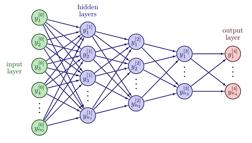
Introducing hidden layers, i.e. layers between the input and output layer, leads to Feedforward Neural Networks (FNNs), also called multilayer perceptrons (MLPs), cf. . Essentially, they are multiple perceptrons organized in layers, [math]\ell = 0, \ldots, L[/math], where every perceptron takes the output from the previous perceptron as input. The number of layers [math]L[/math] is called the depth of the network, while the number of neurons per layer [math]n_\ell[/math] is the width of the network. The input layer is denoted with [math]y^{[0]} = u \in \mathbb{R}^{n_0}[/math] and not counted in the depth of the network. A FNN is called deep if it has at least two hidden layers. We now indicate the weights from layer [math]\ell[/math] to [math]\ell+1[/math] by [math]W^{[\ell]} \in \mathbb{R}^{n_{\ell + 1} \times n_\ell}[/math] and the bias vector by [math]b^{[\ell]} \in \mathbb{R}^{n_{\ell+1}}[/math] for [math]\ell=0,\ldots,L-1[/math]. To simplify notation, we extend the activation function [math]\sigma:\mathbb{R}\rightarrow \mathbb{R}[/math] to vector valued inputs, by applying it component-wise, so that [math]\sigma:\mathbb{R}^n \rightarrow \mathbb{R}^n[/math], with [math](y_1,\ldots,y_n)^{\top} \mapsto (\sigma(y_1),\ldots,\sigma(y_n))^\top[/math]. The FNN layers can be represented in the same way as perceptrons

[[math]] \begin{equation} \label{eq:FNNarchitecture} y^{[\ell]} = f_\ell (y^{[\ell-1]}) = \sigma^{[\ell]} ( W^{[\ell -1]} y^{[\ell-1]} + b^{[\ell-1]} ) \qquad \text{for } \ell=1,\ldots,L, \end{equation} [[/math]]

where the activation function [math]\sigma^{[\ell]}[/math] may differ from layer to layer. We call [math]y^{[\ell]}[/math] the feature vector of layer [math]\ell[/math]. Compactly, we can write a FNN as a composition of its layer functions, cf.

[[math]] y^{[L]} = \mathcal{F}(u) = f_{L} \circ f_{L-2}\circ\ldots \circ f_1(u). [[/math]]

This formulation reinforces the choice of nonlinear activation function [math]\sigma[/math], cf. Remark. Otherwise, the output [math]y^{[L]}[/math] is linearly dependent on the input [math]u[/math] and hidden layers can be eliminated. Hence, with linear activation function, solving rather simple tasks like modeling the logical "XOR" function will not be possible. However, sometimes it can be favorable to have one linear layer.

In practice, it is not uncommon that the last layer of a FNN is indeed linear, i.e. [math]y^{[L]} = W^{[L-1]} y^{[L-1]}[/math]. As long as the previous layers are nonlinear this does not hinder the expressiveness of the FNN, and is typically used to attain a desired output dimension. In essence, [math]W^{[L-1]}[/math] can be seen as a reformatting, in this case.

However, in the remainder of this section we will consider the FNN architecture as introduced in \eqref{eq:FNNarchitecture}. Let us now try again to represent the "XOR" logical function, this time by a FNN with one hidden layer.

A feedforward network with a two dimensional input and one hidden layer with 2 nodes, i.e. [math]n_0 = n_1 = 2, n_2 = 1[/math] and [math]L=2[/math].

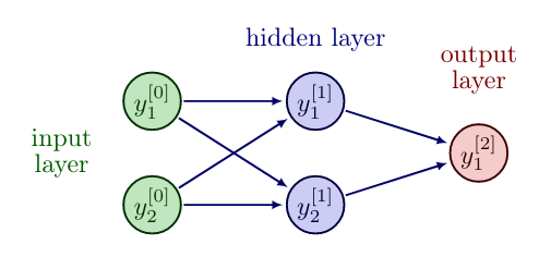
The variable choices

[[math]]W^{[0]} = \begin{pmatrix} 1 & 1 \\ -1 & -1 \end{pmatrix}, \quad b^{[0]} = \begin{pmatrix} -1 \\ 1 \end{pmatrix}, \quad W^{[1]} = \begin{pmatrix} 1 & 1 \end{pmatrix}, \quad b^{[1]} = -2, [[/math]]

solve the task and lead to the following truth table.

Truth table for the logical "XOR" function modeled by the FNN from Figure and given variable choices as above.

input [math]y^{[0]}_1[/math]	input [math]y^{[0]}_2[/math]	[math]y^{[1]}_1[/math]	[math]y^{[1]}_2[/math]	[math]y^{[0]}_1[/math] XOR [math]y^{[0]}_2[/math] (output [math]y^{[2]}_1[/math])
0	0	0	1	0
1	0	1	1	1
0	1	1	1	1
1	1	1	0	0

Next, we formulate an optimization problem similar to eq:LP for multiple layers with the above introduced notation, cf.

[[math]] \begin{align}\label{eq:Pell} \tag{$P_\ell$} &\min_{\{W^{[\ell]}\}_\ell, \{b^{[\ell]}\}_\ell} \mathscr{L}\left(\{y^{[L](i)}\}_i,\{u^{(i)}\}_i, \{W^{[\ell]}\}_\ell, \{b^{[\ell]}\}_\ell \right) \\ &\qquad\; \text{s.t.} \qquad y^{[L](i)} = \mathcal{F}\left( u^{(i)},\{W^{[\ell]}\}_\ell, \{b^{[\ell]}\}_\ell\right). \notag \end{align} [[/math]]

If we collect again all variables in one vector [math]\theta[/math] this will have the following length:

[[math]] \underbrace{n_0\cdot n_1 + \ldots + n_{L-1} \cdot n_L}_{\text{weights}}+\underbrace{n_1 + \ldots + n_L.}_{\text{biases}} [[/math]]

A feedforward network with 3 hidden layers, layer widths [math]n_0 =3, n_1 = n_2 = n_3 = 5, n_4 = 1[/math] and depth [math]L=4[/math]. Collecting all variables of this network in a vector will give [math]\theta \in \mathbb{R}^{86}.[/math]

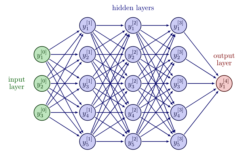
The question that immediately arises is: How to choose the network architecture, i.e. depth and width of the FNN? The following discussion is based on .

Depth and Width

The universal approximation theorem, see e.g. , states that any vector-valued, multivariate, measurable (in particular, continuous) function [math]f:\mathbb{R}^{n_0} \rightarrow \mathbb{R}^{n_L}[/math] can be approximated with arbitrary small error by a Neural Network with one hidden layer. Hence, a first approach may be to choose a network with depth [math]L=2[/math] and increase the width until the desired accuracy is reached.

However, this poses certain problems. First of all the universal approximation theorem does not imply that a training algorithm will actually reach the desired approximation, but rather that some set of parameters exists, that satisfies the requirement. The training algorithm might for example only find a local minimum or choose the wrong function as a result of overfitting. Another problem may be the sheer size of the layer required to achieve the wanted accuracy. In the worst case the network will need an exponential number of hidden units, with one hidden unit for each possible combination of inputs. Thus in practice, one is discouraged to use only one hidden layer, but instead to use deep networks.

Various families of functions are efficiently approximated by deep networks with a smaller width. If one desires to approximate the same function to the same degree of accuracy, the number of hidden units typically grows exponentially. This stems from the fact, that each new layer allows the network to make exponentially more connections, thus allowing a wider output of target functions. Another reason why one might choose deeper networks is due to the intuition, that our desired function may well be a composition of multiple functions. Each new layer adds a nonlinear layer function to our network, thus making it easier for the FNN to approximate composite functions. Also, heuristically we observe that deep networks typically outperform shallow networks.

Nonetheless, one main problem with deep FNNs is, that the gradient used for training is the product of the partial derivatives of each layer, as we will see in Section Backpropagation . If these derivatives have small values, then the gradient for earlier layers can become very small. Thus training has a smaller if not even a negligible effect on the first layers when the network is too deep. This is especially a problem for sigmoid activation function, since its derivative is bounded by [math]\frac{1}{4}[/math].

As discussed in Section Hyperparameters and Data Set Splitting , choosing hyperparameters like the depth and width is a non-trivial undertaking and currently, the method of choice is experimenting to find a suitable configuration for the given task.

Additionally, in the optimization algorithms, cf. Section Optimization Algorithms , we need a starting point [math]\theta^0[/math] for the variables. Hence, we discuss how to initialize the weights and biases in the FNN.

Initialization

Recall that due to the non-convex loss function, we can only expect convergence to stationary points, cf. Remark. Consequently, the choice of the initial point [math]\theta^0[/math] can have great impact on the algorithm, since two different initial points can lead to two different results. An unsuitable initial point may even prevent convergence altogether. Similar to choosing hyperparameters, for the choice of initial points there exist several well-tested strategies, cf. , but it is still an active field of research.

The naive approach would be to initialize [math]\theta = 0[/math] or with some other constant value. Unfortunately, this strategy has major disadvantages. With this initialization, all weights per layer in the Neural Network have the same influence on the loss function and will therefore have the same gradient. This leads to all those neurons evolving symmetrically throughout training, so that different neurons will not learn different things, which significantly reduces the expressiveness of the FNN. Let us remark that it is fine to initialize the biases [math]b^{[\ell]}[/math] with zero, as long as the weights [math]W^{[\ell]}[/math] are not initialized constant. Hence, it is sufficient to discuss initialization strategies for the weights.

We know now that the weights should be initialized in a way that they differ from each other to ensure symmetry breaking, i.e. preventing the neurons from evolving identically. One way to achieve this is random initialization. However, immediately the next question arises: How to generate those random values?

For example, weights can be drawn from a Gaussian distribution with mean zero and some fixed standard deviation. Choosing a small standard deviation, e.g. 0.01, may cause a problem known as vanishing gradients for deep networks, since the small neuron values will be multiplied with each other in the computation of gradients due to the chain rule, leading to exponentially decaying products. As a result learning can be very slow or even diverge. On the other hand, choosing a large standard deviation, e.g. 0.2, can result in exploding gradients, which is essentially the opposite problem, where the products grow exponentially and learning can become unstable, oscillate or even produce "NaN" values for the variables. Furthermore, in combination with saturating activation functions like sigmoid or [math]\tanh[/math] exploding variable values can lead to saturation of the activation function, which then leads to vanishing gradients and again hinder learning, cf. Figure.

To find a good intermediate value for the standard deviation, Xavier initialization has been proposed in , where the standard deviation value is chosen depending on the input size of the layer, i.e.

[[math]]\frac{1}{\sqrt{n_{\ell}}}[[/math]]

for [math]W^{[\ell]}, \ell = 0,\ldots,L-1[/math]. Note that since input sizes can vary, the Gaussian distribution that the initial values are drawn from, will also vary. This choice of weights in combination with [math]b^{[\ell]} = 0[/math] leads to [math]\text{Var}(y^{[\ell+1]}) = \text{Var}(y^{[\ell]})[/math]. However, the Xavier initialization assumes zero centered activation functions, which is not fulfilled for sigmoid and all variants of ReLU. As a remedy, the He initialization has been proposed in , tailored especially to ReLU activation functions. Here, the standard deviation is also chosen depending on the input size of the layer, namely

[[math]]\sqrt{\frac{2}{n_\ell}}.[[/math]]

Additionally, there also exists an approach to normalize feature vectors throughout the network.

Batch Normalization

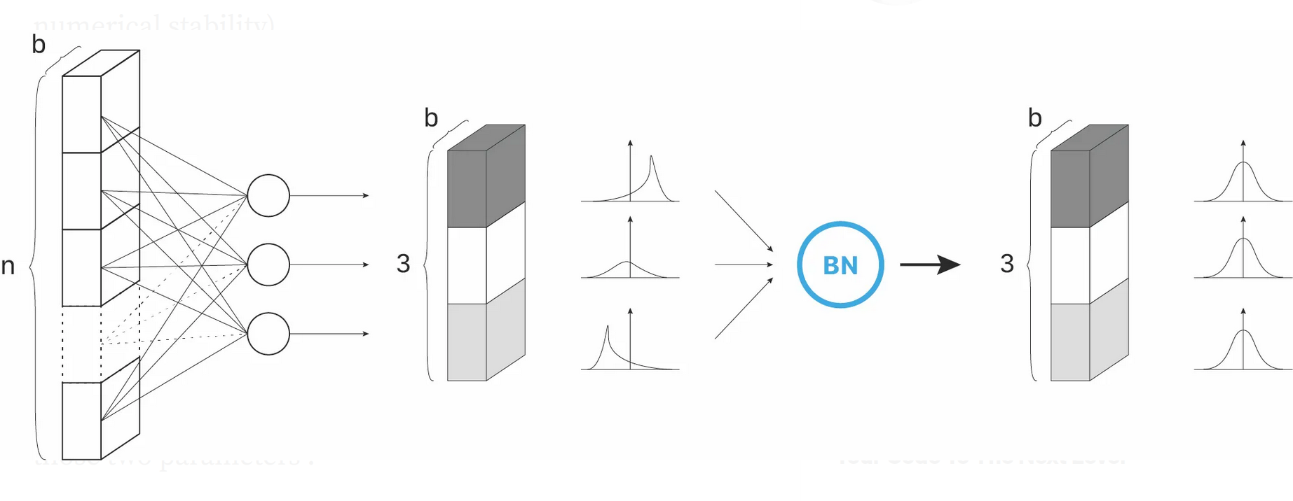
Assume that we are employing an optimization algorithm, which passes through the data points in batches of size [math]b[/math] and that the nodes in hidden layers follow a normal distribution. Then batch normalization aims at normalizing the feature vectors in a hidden layer over the given batch, to stabilize training, especially for unbounded activation functions, such as ReLU. It can be seen as insertion of an additional layer in a deep neural network, and this layer type is already pre-implemented in learning frameworks like tensorflow and pytorch:

• tf.keras.layers.BatchNormalization,
• torch.nn.BatchNorm1d (also 2d and 3d available).

Say, we have given the current feature vectors [math]y^{[\ell]}_j \in \mathbb{R}^{n_\ell}[/math] of hidden layer [math]\ell[/math] for all elements in the batch, i.e. [math]j=1,\ldots,b[/math]. The batch normalzation technique first determines the mean and variance

[[math]] \mu^{[\ell]} = \frac{1}{b} \sum_{j=1}^b y^{[\ell]}_j, \qquad (\sigma^2)^{[\ell]} = \frac{1}{b} \sum_{j=1}^b \left\| y^{[\ell]}_j - \mu^{[\ell]}\right\|^2. [[/math]]

Subsequently, the current feature vectors [math]y^{[\ell]}_j, j = 1,\ldots,b[/math] are normalized via

[[math]] \hat{y}^{[\ell]}_j = \frac{ y_j^{[\ell]}-\mu^{[\ell]} }{ \sqrt{ (\sigma^2)^{[\ell]} + \epsilon }}, [[/math]]

where [math]\epsilon \in \mathbb{R}[/math] is a constant that helps with numerical stability.

Finally, the output of the batch normalization layer is computed by

[[math]] y^{[\ell+1]}_j = W^{[\ell]} \hat{y}^{[\ell]}_j + b^{[\ell]} \qquad \forall \, j=1,\ldots,b.[[/math]]

As usual, the weight [math]W^{[\ell]} \in \mathbb{R}^{n_{\ell+1} \times n_\ell}[/math] and bias [math]b^{[\ell]} \in \mathbb{R}^{n_{\ell +1}}[/math] are variables of the neural network and will be learned.

Illustration of Batch Normalization applied to a hidden layer with 3 nodes and batch size [math]b[/math]. We assume that every node can be modeled by a normal distribution. Image Source: [1].

The BN layer is a trainable layer, since it contains learnable variables.

Let us now consider an example task that is commonly solved with FNNs.

Classification Tasks

As mentioned in Supervised Learning , classification is a supervised learning task with labels [math]S(u) \in \mathbb{N}[/math]. First, we consider binary classification, cf. e.g. , where we classify the data into two categories, i.e. a spam filter that determines whether an email is spam or not. We could construct our network so that it indicates the category which it concludes is the most likely. However, it can be useful to know the probability assigned to the output, so that we know how certain the decision is. Thus, we aim to have outputs between 0 and 1, so that they sum up to 1. In the case of binary classification, the second output is directly determined by the first. Consequently, it suffices to have a one dimensional output layer [math]y^{[L]} \in [0,1][/math], which should predict

[[math]]P(y^{[L]} = 1 \, | \, u, \theta),[[/math]]

i.e. the probability of the output being category 1 (e.g. spam) given the input [math]u[/math] and variables [math]\theta[/math].

Assume that we have already set up a feedforward network up to the second to last layer [math]y^{[L-1]} \in \mathbb{R}[/math]. It remains to choose the activation function [math]\sigma^{[L-1]}[/math] that enters the computation of [math]y^{[L]}[/math] and to model the loss function [math]\mathscr{L}[/math].

File:Guide nna

Let us remark that the cases [math]y^{[L]} \in \{0,1\}[/math] are not possible with this choice of activation function, but we are only computing approximations anyhow.

Next, we construct a loss function. To this end, we assume that the training data is a sample of the actual relationship we are trying to train, thus it obeys a probability function, which we want to recover. The main idea for the loss function is to maximize the likelihood of the input parameters, i.e. if the probability [math]P(y^{[L]} = S(u) \, | \, u,\theta) [/math] of generating the known supervision [math]S(u)[/math] is high for the input data [math]u[/math], the loss should be small, and vice versa. To model the probability we choose the Bernoulli distribution, which models binary classification:

[[math]] P\left(y^{[L]} = S(u) \, | \, u,\theta\right) = (y^{[L]})^{S(u)} (1-y^{[L]})^{(1-S(u))}. [[/math]]

To achieve small loss for large probabilities, we apply the logarithm and then maximize this function, so that the optimal network variables [math]\bar \theta[/math] can be determined as follows

[[math]] \begin{align*} \bar{\theta} &= \underset{\theta}{\operatorname{argmax}} \sum_{i=1}^N \log\left(P\left(y^{[L](i)} = S(u^{(i)}) \, | \, u^{(i)},\theta\right)\right) \\ &= \underset{\theta}{\operatorname{argmax}} \sum_{i=1}^N \log\left( (y^{[L](i)})^{S(u^{(i)})} (1-y^{[L](i)})^{(1-S(u^{(i)}))} \right)\\ &= \underset{\theta}{\operatorname{argmax}} \sum_{i=1}^N S(u^{(i)}) \cdot \log(y^{[L](i)}) + (1-S(u^{(i)})) \cdot \log(1-y^{[L](i)}) \\ &= \underset{\theta}{\operatorname{argmin}} \sum_{i=1}^N \underbrace{- S(u^{(i)}) \cdot \log(y^{[L](i)}) - (1-S(u^{(i)})) \cdot \log(1-y^{[L](i)})}_{=: \mathcal{L}\left(y^{[L](i)},S(u^{(i)})\right), \; '''Binary Cross Entropy Loss'''}, \end{align*} [[/math]]

where [math]y^{[L](i)}[/math] is a function of the network variables [math]\theta[/math].

In practice, we minimize the cross-entropy, since it is equivalent to maximizing the likelihood, but stays within our given frame of minimization problems. Let us assume that our data either has the label [math]S(u)= 1[/math] (spam) or [math]S(u) = 0[/math] (not spam), then the binary cross entropy loss is

[[math]] \mathscr{L}\left(y^{[L]},S(u)\right) = \begin{cases} -\log(y^{[L]}), &\text{if } S(u) = 1, \\ -\log(1-y^{[L]}), &\text{if } S(u) = 0. \end{cases} [[/math]]

Binary Cross Entropy Loss for label [math]S(u) = 1[/math] (left) and label [math]S(u)=0[/math] (right).

We see in Figure that the cross entropy loss for [math]S(u)=1[/math] goes to zero, for [math]y^{[L]} \nearrow 1[/math], and grows for [math]y^{[L]} \searrow 0[/math], as desired. On the other hand, the cross entropy loss for [math]S(u)=0[/math] goes to zero for [math]y^{[L]} \searrow 0[/math] and grows for [math]y^{[L]} \nearrow 1[/math].

Altogether, we have the following loss function for the binary classification task

[[math]] \mathscr{L}(\theta) = \frac{1}{N} \sum_{i=1}^N \mathcal{L}\left(y^{[L](i)}(\theta),S(u^{(i)})\right) .[[/math]]

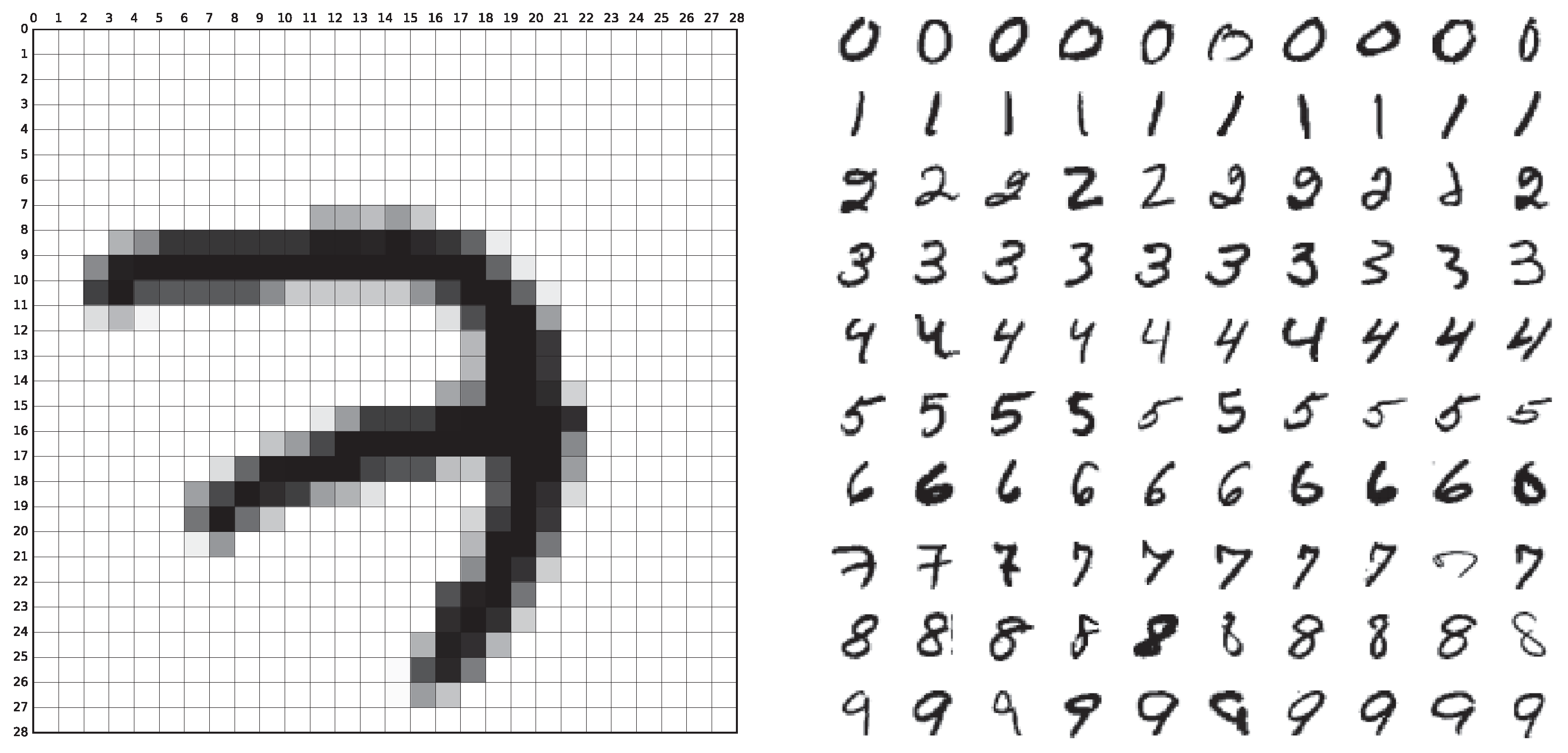
Multiclass classification is a direct extension of binary classification. Here, the goal is to classify the data into multiple (at least 3) categories. A prominent example is the MNIST data set, where black and white pictures of handwritten digits (of size [math]28 \times 28[/math] pixels) are supposed to be classified as [math]\{0,1,2,3,4,5,6,7,8,9\}[/math], cf. Figure. A possible network architecture is illustrated in Figure.

Example of the MNIST database. Sample belonging to the digit 7 (left) and 100 samples from all 10 classes (right). Image Source: .

A feedforward network with 3 hidden layers, i.e. depth [math]L=4[/math]. For the MNIST data set we have [math]n_0 = 784[/math] and [math]n_4 = 10[/math].

For this task, we need a generalization of the sigmoid activation function, which will take [math]y^{[L-1]} \in \mathbb{R}^{n}[/math] and map it to [math]y^{[L]} \in [0,1]^n[/math], so that we have [math]\sum_{i=1}^n y^{[L]}_i = 1[/math], where [math]n_{L-1} = n_L = n[/math] is the number of classes. A suitable option is the softmax function, which is given component-wise by

[[math]] \operatorname{softmax}(y)_i = \frac{\exp(y_i)}{\sum_{j=1}^n \exp(y_j)} \in (0,1), \qquad \text{for } i = 1, \ldots, n. [[/math]]

Keep in mind that e.g. in the MNIST case we have labels [math]S(u) \in \{0,1,2,3,4,5,6,7,8,9\}[/math], and in general we have multiple labels [math]S(u) \in \mathbb{N}[/math]. We have seen before that maximizing the log-likelihood is a suitable choice for classification tasks. Since we want to formulate a minimization problem, we choose the negative log-likelihood as loss function

[[math]] \mathscr{L} (\theta) = \frac{1}{N} \sum_{1=1}^N - \log \left(P\left(y^{[L](i)} = S(u^{(i)}) \, | \, u^{(i)},\theta\right)\right). [[/math]]

In this section we have seen yet another model for the loss function [math]\mathscr{L}[/math], and from Section Optimization Algorithms we know that in any case we will need the gradient [math]\nabla \mathscr{L}(\theta)[/math] to update our variables [math]\theta[/math]. Let us discuss how frameworks like pytorch and tensorflow obtain this information.

Backpropagation

The derivations are based on and . When a network, e.g. a FNN, takes an input [math]u[/math], passes it through its layers and finally computes an output [math]y^{[L]}[/math], the network feeds forward the information, which this is called forward propagation. Then a loss is assigned to the output and we aim at employing the gradient of the loss function [math]\nabla \mathscr{L}(\theta)[/math] to update the network variables [math] \theta \in \mathbb{R}^K[/math]. In a FNN we have [math]K = n_0\cdot n_1 + \ldots + n_{L-1} \cdot n_L+n_1 + \ldots + n_L. [/math] The gradient is then given by

[[math]] \begin{equation*} \nabla \mathscr{L}(\theta) = \begin{pmatrix} \frac{\partial \mathscr{L}(\theta)}{\partial \theta_1} \\ \vdots \\ \frac{\partial \mathscr{L}(\theta)}{\partial \theta_K} \end{pmatrix}. \end{equation*} [[/math]]

To develop an intuition about the process, we discuss the following simple example.

A feedforward network with 2 hidden layers, one node per layer and depth [math]L=3[/math].

Example

Consider a very simple FNN with one node per layer and assume that we only consider weights [math]W^{[\ell]} \in \mathbb{R}[/math] and no biases. For the network in Figure we have [math]\theta = (W^{[0]},W^{[1]},W^{[2]})^{\top}[/math],

[[math]] y^{[3]} = \sigma^{[3]}(W^{[2]}y^{[2]}) = \sigma^{[3]}\left(W^{[2]} \sigma^{[2]} (W^{[1]} y^{[1]}) \right) = \sigma^{[3]}\left(W^{[2]} \sigma^{[2]} \left(W^{[1]} \sigma^{[1]}(W^{[0]}y^{[0]})\right) \right), [[/math]]

and

[[math]] \mathscr{L}(\theta) = \mathscr{L}(y^{[3]}(\theta))= \mathscr{L} \left(\sigma^{[3]}\left(W^{[2]} \sigma^{[2]} \left(W^{[1]} \sigma^{[1]}(W^{[0]}y^{[0]})\right) \right)\right) .[[/math]]

Computing the components of the gradient, we employ the chain rule to obtain e.g.

[[math]] \begin{align*} \frac{\partial \mathscr{L}}{\partial W^{[0]}} &= \frac{\partial \mathscr{L}}{\partial y^{[3]}} \cdot \frac{\partial y^{[3]}}{\partial W^{[0]}} \\ &= \frac{\partial \mathscr{L}}{\partial y^{[3]}} \cdot \frac{\partial y^{[3]}}{\partial y^{[2]}} \cdot \frac{\partial y^{[2]}}{\partial W^{[0]}}\\ &= \frac{\partial \mathscr{L}}{\partial y^{[3]}} \cdot \frac{\partial y^{[3]}}{\partial y^{[2]}} \cdot \frac{\partial y^{[2]}}{\partial y^{[1]}} \cdot \frac{\partial y^{[1]}}{\partial W^{[0]}}, \end{align*} [[/math]]

and in general for depth [math]L[/math] we get

[[math]]\frac{\partial \mathscr{L}}{\partial W^{[\ell]}} = \frac{\partial \mathscr{L}}{\partial y^{[L]}} \cdot \prod_{j=L}^{\ell+2} \frac{\partial y^{[j]}}{\partial y^{[j-1]}} \cdot \frac{\partial y^{[\ell+1]}}{\partial W^{[\ell]}}.[[/math]]

Essentially, to calculate the effect of a variable on the loss function we iterate backwards through the network, multiplying the derivatives of each layer. This is called back propagation, often abbreviated as backprop.

To obtain a computationally efficient version of back propagation, we exploit the fact that parts of the derivatives can be recycled, broadly speaking. E.g. [math] \frac{\partial \mathscr{L}} {\partial y^{[L]}}[/math] is a part of all derivatives. So, if we compute the derivative by [math]W^{[L-1]}[/math] first, we already have this component available and can reuse it in the computation of the derivative by [math]W^{[L-2]}[/math], etc.

In order to formalize the effective computation of derivatives in a backpropagation algorithm, we decompose the forward propagation into two parts, cf. e.g. .

[[math]] \begin{align*} \hspace{4cm} z^{[\ell]} &= W^{[\ell-1]}y^{[\ell-1]} + b^{[\ell-1]} &&\in \mathbb{R}^{n_\ell}, \hspace{4cm} \\ y^{[\ell]} &= \sigma^{\ell]}(z^{[\ell]}) &&\in \mathbb{R}^{n_\ell}. \end{align*} [[/math]]

This was not necessary in Example, because we only consider weights and no biases. Furthermore, we assume that the loss function [math]\mathscr{L}[/math] takes the final output [math]y^{[L]}[/math] as an input. Especially, no other feature vectors [math]y^{[\ell]}[/math] for [math]\ell\neq L[/math] enter the loss function directly. This is the case e.g. for mean squared error, cf. Example, and cross entropy, cf. Section Classification Tasks .

In general, we now have by chain rule for all [math]\ell=0,\ldots,L-1[/math]

[[math]] \begin{align} \frac{\partial \mathscr{L}}{\partial W^{[\ell]}} &= \frac{\partial \mathscr{L}}{\partial y^{[L]}} \cdot \prod_{j=L}^{\ell+2} \left( \frac{\partial y{[j]}}{\partial z^{[j]}} \cdot \frac{\partial z^{[j]}}{\partial y^{[j-1]}} \right) \cdot \frac{\partial y^{[\ell+1]}}{\partial z^{[\ell + 1]}} \cdot \frac{\partial z^{[\ell+1]}}{\partial W^{[\ell]}} , \label{eq:chainW} \\ \frac{\partial \mathscr{L}}{\partial b^{[\ell]}} &= \frac{\partial \mathscr{L}}{\partial y^{[L]}} \cdot \prod_{j=L}^{\ell+2} \left( \frac{\partial y{[j]}}{\partial z^{[j]}} \cdot \frac{\partial z^{[j]}}{\partial y^{[j-1]}} \right) \cdot \frac{\partial y^{[\ell+1]}}{\partial z^{[\ell + 1]}} \cdot \frac{\partial z^{[\ell+1]}}{\partial b^{[\ell]}} \label{eq:chainb}. \end{align} [[/math]]

However, we have to understand these derivatives in detail. First of all, let us introduce the following definition from .

Definition

Let [math]A,B \in \mathbb{R}^{m\times n}[/math] be given matrices, then [math]A \odot B \in \mathbb{R}^{m \times n}[/math], with entries

[[math]] (A\odot B)_{i,j} := (A)_{i,j} \cdot (B)_{i,j}, \qquad \text{for } i=1,\ldots,m, \, j=1,\ldots,n,[[/math]]

is called the Hadamard product of [math]A[/math] and [math]B[/math].

Furthermore, we define the derivative of the component-wise activation function [math]\sigma: \mathbb{R}^m \rightarrow \mathbb{R}^m[/math] as follows

[[math]] \begin{equation*} \sigma' : \mathbb{R}^{m} \rightarrow \mathbb{R}^{m}, \qquad z= \begin{pmatrix} z_1 \\ \vdots \\ z_m \end{pmatrix} \mapsto \begin{pmatrix} \sigma'(z_1) \\ \vdots \\ \sigma'(z_m) \end{pmatrix} = \sigma'(z). \end{equation*} [[/math]]

Let us introduce two special cases of multi-dimensional chain rule, cf. , which will prove helpful to calculate the derivatives.

• Consider [math]a = \sigma(z) \in \mathbb{R}^m[/math], where [math]\sigma[/math] is a component-wise function, e.g. an activation function, [math]z \in \mathbb{R}^m[/math], and [math]f = f(a) \in \mathbb{R}[/math]. Then, it holds
  [[math]] \begin{equation} \; \frac{\partial f}{\partial z} = \frac{\partial f}{\partial a} \odot \sigma'(z) \;\; \in \mathbb{R}^{m}. \label{eq:case1} \end{equation} [[/math]]
• Consider [math]z = W y + b \in \mathbb{R}^m[/math] and [math]f = f(z) \in \mathbb{R}[/math], with [math]W \in \mathbb{R}^{m\times n}[/math] and [math]y \in \mathbb{R}^n[/math]. Then, it holds
  [[math]] \begin{align} \hspace{4.5cm} \frac{\partial f}{\partial y} &= W^{\top} \cdot \frac{\partial f} {\partial z} &&\in \mathbb{R}^{n}, \hspace{4.5cm} \label{eq:case2a}\\ \frac{\partial f}{\partial W} &= \frac{\partial f} {\partial z} \cdot y^{\top} &&\in \mathbb{R}^{m\times n}, \label{eq:case2b}\\ \frac{\partial f}{\partial b} &= \frac{\partial f} {\partial z} &&\in \mathbb{R}^m. \label{eq:case2c} \end{align} [[/math]]

We can now start working our way backwards through the network to get all derivatives. Assume that we know [math]\frac{\partial \mathscr{L}} {\partial y^{[L]}} \in \mathbb{R}^{n_L}[/math], which will depend in detail on the choice of loss function. We can employ \eqref{eq:case1} with [math]f = \mathscr{L}, z = z^{[L]}, a = y^{[L]} [/math] to compute

[[math]] \begin{equation*} \bar{z}^{[L]} := \frac{\partial \mathscr{L}}{\partial z^{[L]}} = \frac{\partial \mathscr{L}}{\partial y^{[L]}} \odot (\sigma^{[L]})'(z^{[L]}) \qquad \in \mathbb{R}^{n_L}. \end{equation*} [[/math]]

Here, we employ a typical notation from automatic differentiation (AD), i.e. the gradient of the loss with respect to a certain variable is denoted by the name of that variable with an overbar. Now, we know

[[math]] \begin{equation*} \bar{y}^{[L-1]} := \frac{\partial \mathscr{L}}{\partial y^{[L-1]}} = \bar{z}^{[L]} \cdot \frac{\partial z^{[L]}}{\partial y^{[L-1]}} \qquad \in \mathbb{R}^{n_{L-1}}, \end{equation*} [[/math]]

i.e. we can reuse the previously derived gradient. Furthermore, from \eqref{eq:case2a} with [math]f = \mathscr{L}[/math], [math]y = y^{[L-1]}, W = W^{[L-1]}, z = z^{[L]}[/math] we deduce

[[math]] \begin{equation*} \bar{y}^{[L-1]} = (W^{[L-1]})^{\top}\bar{z}^{[L]}. \end{equation*} [[/math]]

Subsequently, we use [math]\bar{y}^{[L-1]}[/math] to compute [math]\bar{z}^{[L-1]}[/math], and so forth. In this way we can keep iterating to build up the products in \eqref{eq:chainW} and \eqref{eq:chainb}.

In every layer,[math]\ell=0,\ldots,L-1[/math], we also want to determine [math]\bar{W}^{[\ell]}:= \frac{\partial \mathscr{L}}{\partial W^{[\ell]}} [/math] and [math]\bar{b}^{[\ell]}:= \frac{\partial \mathscr{L}}{\partial b^{[\ell]}}[/math]. We show this exemplary for [math]\ell = L-1[/math]. It holds

[[math]] \begin{align*} \bar{W}^{[L-1]} &= \bar{z}^{[L]} \cdot \frac{\partial z^{[L]}}{\partial W^{[L-1]}} \qquad \in \mathbb{R}^{n_L \times n_{L-1}}, \\ \bar{b}^{[L-1]} &= \bar{z}^{[L]} \cdot \frac{\partial z^{[L]}}{\partial b^{[L-1]}} \qquad\;\,\, \in \mathbb{R}^{n_{L}}. \end{align*} [[/math]]

Making use of \eqref{eq:case2b} and \eqref{eq:case2c} with the same choices as in the computation of [math]\bar{y}^{[L-1]}[/math] and [math]b = b^{[L-1]}[/math], we get

[[math]] \begin{align*} \bar{W}^{[L-1]} &= \bar{z}^{[L]} (y^{[L-1]})^{\top} , \\ \bar{b}^{[L-1]} &= \bar{z}^{[L]}. \end{align*} [[/math]]

With this technique, we have an iterative way to efficiently calculate all gradients needed for the variable update in the optimization method, cf. Section Optimization Algorithms .

• It is even more elegant and efficient to update [math]W^{[\ell]}[/math] and [math]b^{[\ell]}[/math] during backpropagation, i.e. on the fly. This way we do not need to store the gradient and can overwrite the weight and bias variables. It is only necessary to save the current gradients for the next loop, so we could rewrite the backpropagation algorithm with temporary gradient values. This only works if the stepsize / learning rate [math]\tau[/math] is previously known and fixed for all variables, since for a line search we would need to know the full gradient and could only update the variables afterwards.
• Considering we have [math]N[/math] training data points, the backpropagation algorithm has to take all of them into account. When the loss is a sum of loss functions for each data point, this can be easily incorporated into the algorithm by looping over [math]i=1,\ldots,N[/math] and introducing a sum where necessary.

Altogether, we formulate Algorithm Backpropagation, which collects the gradients with respect to the weights and biases in one final gradient vector [math]\nabla \mathscr{L} (\theta)[/math].

Backpropagation

Require: Training data set [math]\{u^{(i)}, S(u^{(i)})\}_{i=1}^N[/math].

Require: Current weights [math]W^{[\ell]}[/math] and biases [math]b^{[\ell]}[/math] for [math]\ell=0,\ldots,L-1[/math].

Require: Activation functions [math]\sigma^{[\ell]}[/math] for [math]\ell=1,\ldots,L[/math].

Require: Loss function [math]\mathscr{L}(y^{[L]})[/math] and its gradient [math]\nabla \mathscr{L}(y^{[L]}) = \frac{\partial \mathscr{L}} {\partial y^{[L]}} \in \mathbb{R}^{n_L}[/math].

[math]y^{[0](i)} = u^{(i)} \in \mathbb{R}^{n_0} \quad[/math] for [math]i = 1, \ldots,N[/math].

for [math]\ell=1,\ldots,L[/math] do

[math]z^{[\ell](i)} = W^{[\ell-1]}y^{[\ell-1]} + b^{[\ell-1]} \in \mathbb{R}^{n_\ell} \quad[/math] for [math]i = 1, \ldots,N[/math],

[math]y^{[\ell](i)} = \sigma^{[\ell]}(z^{[\ell](i)}) \in \mathbb{R}^{n_\ell} \quad[/math] for [math]i = 1, \ldots,N[/math].

end for

Compute loss [math]\mathscr{L} = \frac{1}{N} \sum_{1=1}^N \mathscr{L}(y^{[L](i)}) \in \mathbb{R}[/math].

[math]\bar{y}^{[L](i)} = \frac{1}{N} \cdot \nabla \mathscr{L}(y^{[L](i)} ) \in \mathbb{R}^{ n_L} \quad[/math] for [math]i = 1, \ldots,N[/math].

for [math]\ell = L,L-1,\ldots,1[/math] do

[math]\bar{z}^{[\ell](i)} \hspace{0.36cm} = \bar{y}^{[\ell](i)} \odot (\sigma^{[\ell]})' (z^{[\ell](i)}) \hspace{0.24cm} \in \mathbb{R}^{n_\ell} \quad[/math] \hspace{0.19cm} for [math]i = 1, \ldots,N[/math],

[math]\bar{y}^{[\ell-1](i)} = (W^{[\ell-1]})^{\top}\bar{z}^{[\ell](i)} \in \mathbb{R}^{n_{\ell-1}} \quad[/math] for [math]i = 1, \ldots,N[/math],

[math]\bar{W}^{[\ell-1]} \hspace{0.13cm} = \sum_{1=1}^N \bar{z}^{[\ell](i)} (y^{[\ell-1](i)})^{\top} \in \mathbb{R}^{ n_\ell \times n_{\ell-1}}[/math],

[math]\bar{b}^{[\ell-1]} \hspace{0.37cm} = \sum_{1=1}^N \bar{z}^{[\ell](i)} \in \mathbb{R}^{n_\ell}[/math].

end for

In frameworks like pytorch and tensorflow, backpropagation is already implemented, e.g. in pytorch the function "autograd" handles the backward pass. Broadly speaking, autograd collects the data and all executed operations in a directed acyclic graph. In this graph the inputs are the leaves, while the outputs are the roots. Now to automatically compute the gradients, the graph can be traced from roots to leaves, employing the chain rule. This coincides with the computations that we just derived by hand. For more details we refer to [2].

General references

Herberg, Evelyn (2023). "Lecture Notes: Neural Network Architectures". arXiv:2304.05133 [cs.LG].

References

- 1.0 1.1 1.2 I. Goodfellow, Y. Bengio, and A. Courville. (2016). Deep learning. MIT Press.CS1 maint: multiple names: authors list (link)
- 2.0 2.1 H. Antil, T. S. Brown, R. Löhner, F. Togashi, and D. Verma. (2022). "Deep Neural Nets with Fixed Bias Configuration". arXiv preprint arXiv:2107.01308.
- 3.0 3.1 H. Antil and H. Díaz and E. Herberg (2022). "An Optimal Time Variable Learning Framework for Deep Neural Networks". arXiv preprint arXiv:2204.08528.
- H. Antil, R. Khatri, R. Löhner, and D. Verma. (2020). "Fractional deep neural network via constrained optimization". Machine Learning: Science and Technology 2. IOP Publishing.
- Cybenko, G. (1989). "Approximation by superpositions of a sigmoidal function". Mathematics of control, signals and systems 2. Springer.
- 6.0 6.1 Geiger, A. (2021), Deep Learning Lecture Notes
- Glorot, X. and Bengio, Y. (2010). "Understanding the difficulty of training deep feedforward neural networks". Proceedings of the thirteenth international conference on artificial intelligence and statistics. JMLR Workshop and Conference Proceedings.CS1 maint: uses authors parameter (link)
- He, K. and Zhang, X. and Ren, S. and Sun, J. (2015). "Delving deep into rectifiers: Surpassing human-level performance on imagenet classification". Proceedings of the IEEE international conference on computer vision.CS1 maint: uses authors parameter (link)
- S. Ioffe and C. Szegedy. (2015). "Batch normalization: Accelerating deep network training by reducing internal covariate shift". International conference on machine learning. pmlr.CS1 maint: uses authors parameter (link)
- Baldominos, A. and Saez, Y. and Isasi, P. (2019). "A Survey of Handwritten Character Recognition with MNIST and EMNIST". Applied Sciences 9. doi:.
- 11.0 11.1 11.2 Ng, A. (2022), CS229 Lecture Notes (PDF)
- R. A. Horn. (1990). "The hadamard product". Proc. Symp. Appl. Math 40.