Law of Large Numbers for Continuous Random Variables
In the previous section we discussed in some detail the Law of Large Numbers for discrete probability distributions. This law has a natural analogue for continuous probability distributions, which we consider somewhat more briefly here.
Chebyshev Inequality
Just as in the discrete case, we begin our discussion with the Chebyshev Inequality.
(Chebyshev Inequality) Let [math]X[/math] be a continuous random variable with density function [math]f(x)[/math]. Suppose [math]X[/math] has a finite expected value [math]\mu = E(X)[/math] and finite variance [math]\sigma^2 = V(X)[/math]. Then for any positive number [math]\epsilon \gt 0[/math] we have
The proof is completely analogous to the proof in the discrete case, and we omit it.
Example Let [math]X[/math] be any continuous random variable with [math]E(X) = \mu[/math] and [math]V(X) = \sigma^2[/math]. Then, if [math]\epsilon = k\sigma = k[/math] standard deviations for some integer [math]k[/math], then
just as in the discrete case.
Law of Large Numbers
With the Chebyshev Inequality we can now state and prove the Law of Large Numbers for the continuous case.
(Law of Large Numbers) Let [math]X_1[/math], [math]X_2[/math], \dots, [math]X_n[/math] be an independent trials process with a continuous density function [math]f[/math], finite expected value [math]\mu[/math], and finite variance [math]\sigma^2[/math]. Let [math]S_n = X_1 + X_2 +\cdots+ X_n[/math] be the sum of the [math]X_i[/math]. Then for any real number [math]\epsilon \gt 0[/math] we have
Note that this theorem is not necessarily true if [math]\sigma^2[/math] is infinite (see Example). As in the discrete case, the Law of Large Numbers says that the average value of [math]n[/math] independent trials tends to the expected value as [math]n \to \infty[/math], in the precise sense that, given [math]\epsilon \gt 0[/math], the probability that the average value and the expected value differ by more than [math]\epsilon[/math] tends to 0 as [math]n \to \infty[/math]. Once again, we suppress the proof, as it is identical to the proof in the discrete case.
Uniform Case
Example Suppose we choose at random [math]n[/math] numbers from the interval [math][0,1][/math] with uniform distribution. Then if [math]X_i[/math] describes the [math]i[/math]th choice, we have
Hence,
and for any [math]\epsilon \gt 0[/math],
This says that if we choose [math]n[/math] numbers at random from [math][0,1][/math], then the chances are better than [math]1 - 1/(12n\epsilon^2)[/math] that the difference [math]|S_n/n - 1/2|[/math] is less than [math]\epsilon[/math]. Note that [math]\epsilon[/math] plays the role of the amount of error we are willing to tolerate: If we choose [math]\epsilon = 0.1[/math], say, then the chances that [math]|S_n/n - 1/2|[/math] is less than 0.1 are better than [math]1 - 100/(12n)[/math]. For [math]n = 100[/math], this is about .92, but if [math]n = 1000[/math], this is better than .99 and if [math]n = 10,00[/math], this is better than .999.
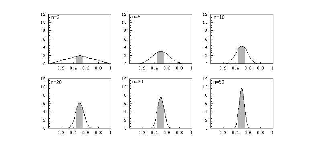
We can illustrate what the Law of Large Numbers says for this example graphically. The density for [math]A_n = S_n/n[/math] is determined by
We have seen in Section \ref{sec 7.2}, that we can compute the density [math]f_{S_n}(x)[/math] for the sum of [math]n[/math] uniform random variables. In Figure we have used this to plot the density for [math]A_n[/math] for various values of [math]n[/math]. We have shaded in the area for which [math]A_n[/math] would lie between .45 and .55. We see that as we increase [math]n[/math], we obtain more and more of the total area inside the shaded region. The Law of Large Numbers tells us that we can obtain as much of the total area as we please inside the shaded region by choosing [math]n[/math] large enough (see also Figure).
Normal Case
Example Suppose we choose [math]n[/math] real numbers at random, using a normal distribution with mean 0 and variance 1. Then
Hence,
and, for any [math]\epsilon \gt 0[/math],
In this case it is possible to compare the Chebyshev estimate for [math]P(|S_n/n - \mu| \geq \epsilon)[/math] in the Law of Large Numbers with exact values, since we know the density function for [math]S_n/n[/math] exactly (see Example). The comparison is shown in Table, for [math]\epsilon = .1[/math]. The data in this table was produced by the program LawContinuous.
| [math]n[/math] | [math]P(|S_n/n| \ge .1)[/math] | Chebyshev |
| 100 | .31731 | 1.00000 |
| 200 | .15730 | .50000 |
| 300 | .08326 | .33333 |
| 400 | .04550 | .25000 |
| 500 | .02535 | .20000 |
| 600 | .01431 | .16667 |
| 700 | .00815 | .14286 |
| 800 | .00468 | .12500 |
| 900 | .00270 | .11111 |
| 1000 | .00157 | .10000 |
We see here that the Chebyshev estimates are in general not very accurate.
Monte Carlo Method
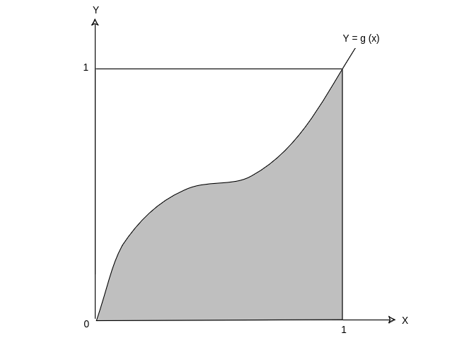
Here is a somewhat more interesting example. Example Let [math]g(x)[/math] be a continuous function defined for [math]x \in [0,1][/math] with values in [math][0,1][/math]. In Simulation of Continuous Probabilities, we showed how to estimate the area of the region under the graph of [math]g(x)[/math] by the Monte Carlo method, that is, by choosing a large number of random values for [math]x[/math] and [math]y[/math] with uniform distribution and seeing what fraction of the points [math]P(x,y)[/math] fell inside the region under the graph (see Example).
Here is a better way to estimate the same area (see Figure). Let us choose a
large number of independent values [math]X_n[/math] at random from [math][0,1][/math] with uniform
density, set [math]Y_n = g(X_n)[/math], and find the average value of the [math]Y_n[/math]. Then
this average is our estimate for the area. To see this, note that if the
density function for [math]X_n[/math] is uniform,
This says that to get within [math]\epsilon[/math] of the true value for [math]\mu = \int_0^1 g(x)\, dx[/math] with probability at least [math]p[/math], we should choose [math]n[/math] so that [math]1/n\epsilon^2 \leq 1 - p[/math] (i.e., so that [math]n \geq 1/\epsilon^2(1 - p)[/math]). Note that this method tells us how large to take [math]n[/math] to get a desired accuracy.
The Law of Large Numbers requires that the variance [math]\sigma^2[/math] of the original underlying density be finite: [math]\sigma^2 \lt \infty[/math]. In cases where this fails to hold, the Law of Large Numbers may fail, too. An example follows.
Cauchy Case
Example Suppose we choose [math]n[/math] numbers from [math](-\infty,+\infty)[/math] with a Cauchy density with parameter [math]a = 1[/math]. We know that for the Cauchy density the expected value and variance are undefined (see Example). In this case, the density function for
General references
Doyle, Peter G. (2006). "Grinstead and Snell's Introduction to Probability" (PDF). Retrieved June 6, 2024.

