Continuous Random Variables
In this section we consider the properties of the expected value and the variance of a continuous random variable. These quantities are defined just as for discrete random variables and share the same properties.
Expected Value
Let [math]X[/math] be a real-valued random variable with density function [math]f(x)[/math]. The expected value [math]\mu = E(X)[/math] is defined by
The reader should compare this definition with the corresponding one for discrete random variables in Expected Value. Intuitively, we can interpret [math]E(X)[/math], as we did in the previous sections, as the value that we should expect to obtain if we perform a large number of independent experiments and average the resulting values of [math]X[/math].
We can summarize the properties of [math]E(X)[/math] as follows (cf. Theorem).
If [math]X[/math] and [math]Y[/math] are real-valued random variables and [math]c[/math] is any constant, then
The proof is very similar to the proof of Theorem, and we omit it.
More generally, if [math]X_1[/math], [math]X_2[/math], \dots, [math]X_n[/math] are [math]n[/math] real-valued random
variables, and
[math]c_1[/math], [math]c_2[/math], \dots, [math]c_n[/math] are [math]n[/math] constants, then
Example Let [math]X[/math] be uniformly distributed on the interval [math][0, 1][/math]. Then
It follows that if we choose a large number [math]N[/math] of random numbers from [math][0,1][/math] and take the average, then we can expect that this average should be close to the expected value of 1/2.
Example Let [math]Z = (x, y)[/math] denote a point chosen uniformly and randomly from the unit disk, as in the dart game in randomly from the unit disk, as in the dart game in Example and let [math]X = (x^2 + y^2)^{1/2}[/math] be the distance from [math]Z[/math] to the center of the disk. The density function of [math]X[/math] can easily be shown to equal [math]f(x) = 2x[/math], so by the definition of expected value,
Example In the example of the couple meeting at the Inn (Example), each person arrives at a time which is uniformly distributed between 5:00 and 6:00 PM. The random variable [math]Z[/math] under consideration is the length of time the first person has to wait until the second one arrives. It was shown that
for [math]0 \le z \le 1[/math]. Hence,
Expectation of a Function of a Random Variable
Suppose that [math]X[/math] is a real-valued random variable and [math]\phi(x)[/math] is a continuous function from R to R. The following theorem is the continuous analogue of Theorem.
If [math]X[/math] is a real-valued random variable and if [math]\phi :[/math] R [math]\to\ [/math] R is a continuous real-valued function with domain [math][a,b][/math], then
For a proof of this theorem, see Ross.[Notes 1]
Expectation of the Product of Two Random Variables
In general, it is not true that [math]E(XY) = E(X)E(Y)[/math], since the integral of a product is not the product of integrals. But if [math]X[/math] and [math]Y[/math] are independent, then the expectations multiply.
Let [math]X[/math] and [math]Y[/math] be independent real-valued continuous random variables with finite expected values. Then we have
We will prove this only in the case that the ranges of [math]X[/math] and [math]Y[/math] are contained in the intervals [math][a, b][/math] and [math][c, d][/math], respectively. Let the density functions of [math]X[/math] and [math]Y[/math] be denoted by [math]f_X(x)[/math] and [math]f_Y(y)[/math], respectively. Since [math]X[/math] and [math]Y[/math] are independent, the joint density function of [math]X[/math] and [math]Y[/math] is the product of the individual density functions. Hence
The proof in the general case involves using sequences of bounded random variables that approach [math]X[/math]
and [math]Y[/math], and is somewhat technical, so we will omit it.
In the same way, one can show that if [math]X_1[/math], [math]X_2[/math], \dots, [math]X_n[/math] are [math]n[/math] mutually independent real-valued random variables, then
Example unit square. Let [math]A = X^2[/math] and [math]B = Y^2[/math]. Then Theorem implies that [math]A[/math] and [math]B[/math] are independent. Using Theorem, the expectations of [math]A[/math] and [math]B[/math] are easy to calculate:
Using Theorem, the expectation of [math]AB[/math] is just the product of [math]E(A)[/math] and [math]E(B)[/math], or 1/9. The usefulness of this theorem is demonstrated by noting that it is quite a bit more difficult to calculate [math]E(AB)[/math] from the definition of expectation. One finds that the density function of [math]AB[/math] is
so
Example Again let [math]Z = (X, Y)[/math] be a point chosen at random in the unit square, and let [math]W = X + Y[/math]. Then [math]Y[/math] and [math]W[/math] are not independent, and we have
We turn now to the variance.
Variance
Let [math]X[/math] be a real-valued random variable with density function [math]f(x)[/math]. The variance [math]\sigma^2 = V(X)[/math] is defined by
The next result follows easily from Theorem. There is another way to calculate the variance of a continuous random variable, which is usually slightly easier. It is given in Theorem.
If [math]X[/math] is a real-valued random variable with [math]E(X) = \mu[/math], then
The properties listed in the next three theorems are all proved in exactly the same way that the corresponding theorems for discrete random variables were proved in Variance of Discrete Random Variables.
If [math]X[/math] is a real-valued random variable defined on [math]\Omega[/math] and [math]c[/math] is any constant, then (cf. Theorem)
If [math]X[/math] is a real-valued random variable with [math]E(X) = \mu[/math], then (cf. Theorem)
If [math]X[/math] and [math]Y[/math] are independent real-valued random variables on [math]\Omega[/math], then (cf. Theorem)
Example (continuation of Example) If [math]X[/math] is uniformly distributed on [math][0, 1][/math], then, using Theorem, we have
Example Let [math]X[/math] be an exponentially distributed random variable with parameter [math]\lambda[/math]. Then the density function of [math]X[/math] is
From the definition of expectation and integration by parts, we have
Similarly, using Theorem and Theorem, we have
In this case, both [math]E(X)[/math] and [math]V(X)[/math] are finite if [math]\lambda \gt 0[/math].
Example Let [math]Z[/math] be a standard normal random variable with density function
Since this density function is symmetric with respect to the [math]y[/math]-axis, then it is easy to show that
has value 0. The reader should recall however, that the expectation is defined to be the above integral only if the integral
is finite. This integral equals
which one can easily show is finite. Thus, the expected value of [math]Z[/math] is 0.
To calculate the variance of [math]Z[/math], we begin by applying Theorem:
If we write [math]x^2[/math] as [math]x\cdot x[/math], and integrate by parts, we obtain
The first summand above can be shown to equal 0, since as [math]x \rightarrow \pm \infty[/math], [math]e^{-x^2/2}[/math] gets small more quickly than [math]x[/math] gets large. The second summand is just the standard normal density integrated over its domain, so the value of this summand is 1. Therefore, the variance of the standard normal density equals 1.
Now let [math]X[/math] be a (not necessarily standard) normal random variable with
parameters
[math]\mu[/math] and [math]\sigma[/math]. Then the density function of [math]X[/math] is
We can write [math]X = \sigma Z + \mu[/math], where [math]Z[/math] is a standard normal random variable. Since [math]E(Z) = 0[/math] and [math]V(Z) = 1[/math] by the calculation above, Theorem and Theorem imply that
Example Let [math]X[/math] be a continuous random variable with the Cauchy density function
Then the expectation of [math]X[/math] does not exist, because the integral
diverges. Thus the variance of [math]X[/math] also fails to exist. Densities whose variance is not defined, like the Cauchy density, behave quite differently in a number of important respects from those whose variance is finite. We shall see one instance of this difference in Continuous Random Variables.
Independent Trials
If [math]X_1, X_2, \ldots, X_n[/math] is an independent trials process of real-valued random variables, with [math]E(X_i) = \mu[/math] and [math]V(X_i) = \sigma^2[/math], and if
then
then
Queues
Example Let us consider again the queueing problem, that is,the problem of the customers waiting in a queue for service (see Example). We suppose again that customers join the queue in such a way that the time between arrivals is an exponentially distributed random variable [math]X[/math] with density function
Then the expected value of the time between arrivals is simply [math]1/\lambda[/math] (see Example), as was stated in Example. The reciprocal [math]\lambda[/math] of this expected value is often referred to as the arrival rate. The service time of an individual who is first in line is defined to be the amount of time that the person stays at the head of the line before leaving. We suppose that the customers are served in such a way that the service time is another exponentially distributed random variable [math]Y[/math] with density function
Then the expected value of the service time is
The reciprocal [math]\mu[/math] if this expected value is often referred to as the service rate.
We expect on grounds of our everyday experience with queues that if the service
rate is greater than the arrival rate, then the average queue size will tend to
stabilize, but if the service rate is less than the arrival rate, then the queue will
tend to increase in length without limit (see Figure). The simulations in Example tend to bear out our everyday experience. We can make this conclusion more precise if we introduce the traffic intensity as the product
The traffic intensity is also the ratio of the average service time to the average time between arrivals. If the traffic intensity is less than 1 the queue will perform reasonably, but if it is greater than 1 the queue will grow indefinitely large. In the critical case of [math]\rho = 1[/math], it can be shown that the queue will become large but there will always be times at which the queue is empty.[Notes 2] In the case that the traffic intensity is less than 1 we can consider the length of the queue as a random variable [math]Z[/math] whose expected value is finite,
The time spent in the queue by a single customer can be considered as a random variable [math]W[/math] whose expected value is finite,
Then we can argue that, when a customer joins the queue, he expects to find [math]N[/math] people ahead of him, and when he leaves the queue, he expects to find [math]\lambda T[/math] people behind him. Since, in equilibrium, these should be the same, we would expect to find that
This last relationship is called Little's law for queues.[Notes 3] We will not prove it here. A proof may be found in Ross.[Notes 4] Note that in this case we are counting the waiting time of all customers, even those that do not have to wait at all. In our simulation in Continuous Conditional Probability, we did not consider these customers.
If we knew the expected queue length then we could use Little's law to obtain
the expected waiting time, since
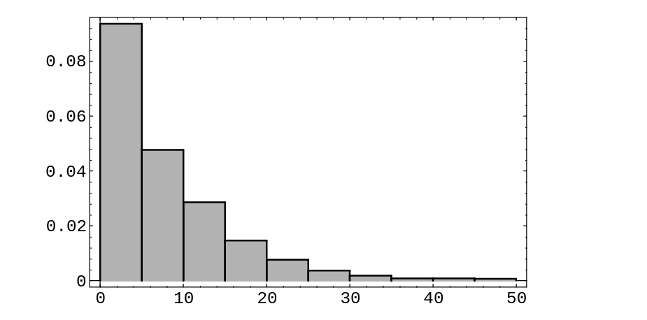
The queue length is a random variable with a discrete distribution. We can estimate this distribution by simulation, keeping track of the queue lengths at the times at which a customer arrives. We show the result of this simulation (using the program Queue) in Figure.
We note that the distribution appears to be a geometric distribution. In the study
of queueing theory it is shown that the distribution for the queue length in equilibrium
is indeed a geometric distribution with
if [math]\rho \lt 1[/math]. The expected value of a random variable with this distribution is
(see Example). Thus by Little's result the expected waiting time is
where [math]\mu[/math] is the service rate, [math]\lambda[/math] the arrival rate, and [math]\rho[/math] the traffic intensity.
In our simulation, the arrival rate is 1 and the service rate is 1.1. Thus, the
traffic intensity is [math]1/1.1 = 10/11[/math], the expected queue size is
and the expected waiting time is
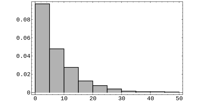
In our simulation the average queue size was 8.19 and the average waiting time was 7.37. In Figure, we show the histogram for the waiting times. This histogram suggests that the density for the waiting times is exponential with parameter [math]\mu - \lambda[/math], and this is the case.
General references
Doyle, Peter G. (2006). "Grinstead and Snell's Introduction to Probability" (PDF). Retrieved June 6, 2024.

