Gradient-Based Learning

[math] % Generic syms \newcommand\defeq{:=} \newcommand{\Tt}[0]{\boldsymbol{\theta}} \newcommand{\XX}[0]{{\cal X}} \newcommand{\ZZ}[0]{{\cal Z}} \newcommand{\vx}[0]{{\bf x}} \newcommand{\vv}[0]{{\bf v}} \newcommand{\vu}[0]{{\bf u}} \newcommand{\vs}[0]{{\bf s}} \newcommand{\vm}[0]{{\bf m}} \newcommand{\vq}[0]{{\bf q}} \newcommand{\mX}[0]{{\bf X}} \newcommand{\mC}[0]{{\bf C}} \newcommand{\mA}[0]{{\bf A}} \newcommand{\mL}[0]{{\bf L}} \newcommand{\fscore}[0]{F_{1}} \newcommand{\sparsity}{s} \newcommand{\mW}[0]{{\bf W}} \newcommand{\mD}[0]{{\bf D}} \newcommand{\mZ}[0]{{\bf Z}} \newcommand{\vw}[0]{{\bf w}} \newcommand{\D}[0]{{\mathcal{D}}} \newcommand{\mP}{\mathbf{P}} \newcommand{\mQ}{\mathbf{Q}} \newcommand{\E}[0]{{\mathbb{E}}} \newcommand{\vy}[0]{{\bf y}} \newcommand{\va}[0]{{\bf a}} \newcommand{\vn}[0]{{\bf n}} \newcommand{\vb}[0]{{\bf b}} \newcommand{\vr}[0]{{\bf r}} \newcommand{\vz}[0]{{\bf z}} \newcommand{\N}[0]{{\mathcal{N}}} \newcommand{\vc}[0]{{\bf c}} \newcommand{\bm}{\boldsymbol} % Statistics and Probability Theory \newcommand{\errprob}{p_{\rm err}} \newcommand{\prob}[1]{p({#1})} \newcommand{\pdf}[1]{p({#1})} \def \expect {\mathbb{E} } % Machine Learning Symbols \newcommand{\biasterm}{B} \newcommand{\varianceterm}{V} \newcommand{\neighbourhood}[1]{\mathcal{N}^{(#1)}} \newcommand{\nrfolds}{k} \newcommand{\mseesterr}{E_{\rm est}} \newcommand{\bootstrapidx}{b} %\newcommand{\modeldim}{r} \newcommand{\modelidx}{l} \newcommand{\nrbootstraps}{B} \newcommand{\sampleweight}[1]{q^{(#1)}} \newcommand{\nrcategories}{K} \newcommand{\splitratio}[0]{{\rho}} \newcommand{\norm}[1]{\Vert {#1} \Vert} \newcommand{\sqeuclnorm}[1]{\big\Vert {#1} \big\Vert^{2}_{2}} \newcommand{\bmx}[0]{\begin{bmatrix}} \newcommand{\emx}[0]{\end{bmatrix}} \newcommand{\T}[0]{\text{T}} \DeclareMathOperator*{\rank}{rank} %\newcommand\defeq{:=} \newcommand\eigvecS{\hat{\mathbf{u}}} \newcommand\eigvecCov{\mathbf{u}} \newcommand\eigvecCoventry{u} \newcommand{\featuredim}{n} \newcommand{\featurelenraw}{\featuredim'} \newcommand{\featurelen}{\featuredim} \newcommand{\samplingset}{\mathcal{M}} \newcommand{\samplesize}{m} \newcommand{\sampleidx}{i} \newcommand{\nractions}{A} \newcommand{\datapoint}{\vz} \newcommand{\actionidx}{a} \newcommand{\clusteridx}{c} \newcommand{\sizehypospace}{D} \newcommand{\nrcluster}{k} \newcommand{\nrseeds}{s} \newcommand{\featureidx}{j} \newcommand{\clustermean}{{\bm \mu}} \newcommand{\clustercov}{{\bm \Sigma}} \newcommand{\target}{y} \newcommand{\error}{E} \newcommand{\augidx}{b} \newcommand{\task}{\mathcal{T}} \newcommand{\nrtasks}{T} \newcommand{\taskidx}{t} \newcommand\truelabel{y} \newcommand{\polydegree}{r} \newcommand\labelvec{\vy} \newcommand\featurevec{\vx} \newcommand\feature{x} \newcommand\predictedlabel{\hat{y}} \newcommand\dataset{\mathcal{D}} \newcommand\trainset{\dataset^{(\rm train)}} \newcommand\valset{\dataset^{(\rm val)}} \newcommand\realcoorspace[1]{\mathbb{R}^{\text{#1}}} \newcommand\effdim[1]{d_{\rm eff} \left( #1 \right)} \newcommand{\inspace}{\mathcal{X}} \newcommand{\sigmoid}{\sigma} \newcommand{\outspace}{\mathcal{Y}} \newcommand{\hypospace}{\mathcal{H}} \newcommand{\emperror}{\widehat{L}} \newcommand\risk[1]{\expect \big \{ \loss{(\featurevec,\truelabel)}{#1} \big\}} \newcommand{\featurespace}{\mathcal{X}} \newcommand{\labelspace}{\mathcal{Y}} \newcommand{\rawfeaturevec}{\mathbf{z}} \newcommand{\rawfeature}{z} \newcommand{\condent}{H} \newcommand{\explanation}{e} \newcommand{\explainset}{\mathcal{E}} \newcommand{\user}{u} \newcommand{\actfun}{\sigma} \newcommand{\noisygrad}{g} \newcommand{\reconstrmap}{r} \newcommand{\predictor}{h} \newcommand{\eigval}[1]{\lambda_{#1}} \newcommand{\regparam}{\lambda} \newcommand{\lrate}{\alpha} \newcommand{\edges}{\mathcal{E}} \newcommand{\generror}{E} \DeclareMathOperator{\supp}{supp} %\newcommand{\loss}[3]{L({#1},{#2},{#3})} \newcommand{\loss}[2]{L\big({#1},{#2}\big)} \newcommand{\clusterspread}[2]{L^{2}_{\clusteridx}\big({#1},{#2}\big)} \newcommand{\determinant}[1]{{\rm det}({#1})} \DeclareMathOperator*{\argmax}{argmax} \DeclareMathOperator*{\argmin}{argmin} \newcommand{\itercntr}{r} \newcommand{\state}{s} \newcommand{\statespace}{\mathcal{S}} \newcommand{\timeidx}{t} \newcommand{\optpolicy}{\pi_{*}} \newcommand{\appoptpolicy}{\hat{\pi}} \newcommand{\dummyidx}{j} \newcommand{\gridsizex}{K} \newcommand{\gridsizey}{L} \newcommand{\localdataset}{\mathcal{X}} \newcommand{\reward}{r} \newcommand{\cumreward}{G} \newcommand{\return}{\cumreward} \newcommand{\action}{a} \newcommand\actionset{\mathcal{A}} \newcommand{\obstacles}{\mathcal{B}} \newcommand{\valuefunc}[1]{v_{#1}} \newcommand{\gridcell}[2]{\langle #1, #2 \rangle} \newcommand{\pair}[2]{\langle #1, #2 \rangle} \newcommand{\mdp}[5]{\langle #1, #2, #3, #4, #5 \rangle} \newcommand{\actionvalue}[1]{q_{#1}} \newcommand{\transition}{\mathcal{T}} \newcommand{\policy}{\pi} \newcommand{\charger}{c} \newcommand{\itervar}{k} \newcommand{\discount}{\gamma} \newcommand{\rumba}{Rumba} \newcommand{\actionnorth}{\rm N} \newcommand{\actionsouth}{\rm S} \newcommand{\actioneast}{\rm E} \newcommand{\actionwest}{\rm W} \newcommand{\chargingstations}{\mathcal{C}} \newcommand{\basisfunc}{\phi} \newcommand{\augparam}{B} \newcommand{\valerror}{E_{v}} \newcommand{\trainerror}{E_{t}} \newcommand{\foldidx}{b} \newcommand{\testset}{\dataset^{(\rm test)} } \newcommand{\testerror}{E^{(\rm test)}} \newcommand{\nrmodels}{M} \newcommand{\benchmarkerror}{E^{(\rm ref)}} \newcommand{\lossfun}{L} \newcommand{\datacluster}[1]{\mathcal{C}^{(#1)}} \newcommand{\cluster}{\mathcal{C}} \newcommand{\bayeshypothesis}{h^{*}} \newcommand{\featuremtx}{\mX} \newcommand{\weight}{w} \newcommand{\weights}{\vw} \newcommand{\regularizer}{\mathcal{R}} \newcommand{\decreg}[1]{\mathcal{R}_{#1}} \newcommand{\naturalnumbers}{\mathbb{N}} \newcommand{\featuremapvec}{{\bf \Phi}} \newcommand{\featuremap}{\phi} \newcommand{\batchsize}{B} \newcommand{\batch}{\mathcal{B}} \newcommand{\foldsize}{B} \newcommand{\nriter}{R} [/math]

This chapter discusses an important family of optimization methods for solving empirical risk minimization (ERM) with a parametrized hypothesis space (see Chapter Computational and Statistical Aspects of ERM ). The common theme of these methods is to construct local approximations of the objective function in ERM. These local approximations are obtained from the gradients of the objective function. Gradient-based methods have gained popularity recently as an efficient technique for tuning the parameters of deep artificial neural network (ANN) (deep net)s within deep learning methods .

Section The Basic Gradient Step discusses gradient descent (GD) as the most basic form of gradient-based methods. The idea of GD is to update the weights by locally optimizing a linear approximation of the objective function. This update is referred to as a GD step and provides the main algorithmic primitive of gradient-based methods. One key challenge for a good use of gradient-based methods is the appropriate extend of the local approximations. This extent is controlled by a step size parameter that is used in the basic GD step. Section Choosing the Learning Rate discusses some approaches for choosing this step size. Section When To Stop? discusses a second main challenge in using gradient-based methods which is to decide when to stop repeating the GD steps.

Section GD for Linear Regression and Section GD for Logistic Regression spell out GD for two instances of ERM arising from linear regression and logistic regression, respectively. The beneficial effect of data normalization on the convergence speed of gradient-based methods is briefly discussed in Section Data Normalization . As explained in Section Stochastic GD , the use of stochastic approximations enables gradient-based methods for applications involving massive amounts of data (“big data”). Section Advanced Gradient-Based Methods develops some intuition for advanced gradient-based methods that exploit the information gathered during previous iterations.

The Basic Gradient Step

Let us rewrite empirical risk minimization (ERM) as the optimization problem

[[math]] \begin{equation} \label{equ_obj_emp_risk_GD} \min_{\weights \in \mathbb{R}^{\featuredim}} f(\weights) \defeq(1/\samplesize) \sum_{\sampleidx=1}^{\samplesize} \loss{(\featurevec^{(\sampleidx)},\truelabel^{(\sampleidx)})}{h^{(\weights)}}. \end{equation} [[/math]]

From now on we tacitly assume that each individual loss

[[math]] \begin{equation} \label{equ_def_componentn_loss_gd} f_{\sampleidx}(\weights) \defeq \loss{(\featurevec^{(\sampleidx)},\truelabel^{(\sampleidx)})}{h^{(\weights)}} \end{equation} [[/math]]

arising in \eqref{equ_obj_emp_risk_GD} represents a differentiable function of the parameter vector [math]\weights[/math]. Trivially, differentiability of the components \eqref{equ_def_componentn_loss_gd} implies differentiability of the overall objective function [math]f(\weights)[/math] \eqref{equ_obj_emp_risk_GD}.

Two important examples of ERM involving such differentiable loss functions are linear regression and logistic regression. In contrast, the hinge loss used by the support vector machine (SVM) results in a non-differentiable objective function [math]f(\weights)[/math] \eqref{equ_obj_emp_risk_GD}. However, it is possible to (significantly) extend the scope of gradient-based methods to non-differentiable functions by replacing the concept of a gradient with that of a subgradient.

Gradient based methods are iterative. They construct a sequence of parameter vectors [math]\weights^{(0)} \rightarrow \weights^{(1)} \dots[/math] that hopefully converge to a minimizer [math]\overline{\weights}[/math] of [math]f(\weights)[/math],

[[math]] \begin{equation} \label{equ_def_opt_weight} f(\overline{\weights}) = \bar{f} \defeq \min_{\weights \in \mathbb{R}^{\featuredim}} f(\weights). \end{equation} [[/math]]

Note that there might be several different optimal parameter vectors [math]\overline{\weights}[/math] that satisfy the optimality condition \eqref{equ_def_opt_weight}. We want the sequence generated by a gradient based method to converge towards any of them. The vectors [math]\weights^{(\itercntr)}[/math] are (hopefully) increasingly, with increasing iteration [math]\itercntr[/math], more accurate approximation for a minimizer [math]\overline{\weights}[/math] of \eqref{equ_def_opt_weight}.

Since the objective function [math]f(\weights)[/math] is differentiable, we can approximate it locally around the vector [math]\weights^{(\itercntr)}[/math] using a tangent hyperplane that passes through the point [math]\big(\weights^{(\itercntr)},f\big(\weights^{(\itercntr)}\big) \big) \in \mathbb{R}^{\featuredim+1}[/math]. The normal vector of this hyperplane is given by [math]\mathbf{n} = (\nabla f\big(\weights^{(\itercntr)}\big) ,-1)[/math] (see Figure fig_smooth_function). The first component of the normal vector is the gradient [math]\nabla f(\weights)[/math] of the objective function [math]f(\weights)[/math] evaluated at the point [math]\weights^{(\itercntr)}[/math]. Our main use of the gradient [math]\nabla f\big(\weights^{(\itercntr)}\big)[/math] will be to construct a linear approximation

[[math]] \begin{equation} \label{equ_linear_approx_diff} f(\weights) \approx f\big(\weights^{(\itercntr)}\big) + \big(\weights-\weights^{(\itercntr)} \big)^{T} \nabla f\big(\weights^{(\itercntr)}\big) \mbox{ for }\weights \mbox{ sufficiently close to } \weights^{(\itercntr)}. \end{equation} [[/math]]

Requiring the objective function [math]f(\weights)[/math] in \eqref{equ_linear_approx_diff} to be differentiable is the same as requiring the validity of the local linear approximation \eqref{equ_linear_approx_diff} at every possible vector [math]\weights^{(\itercntr)}[/math]. It turns out that differentiability alone is not very helpful for the design and analysis of gradient based methods.

Gradient based methods are most useful for finding the minimum of differentiable functions [math]f(\weights)[/math] that are also smooth. Informally, a differentiable function [math]f(\weights)[/math] is smooth if the gradient [math]\nabla f(\weights)[/math] does not change too rapidly as a function of the argument [math]\weights[/math]. A quantitative version of the smoothness concept refers to a function as [math]\beta[/math]-smooth if its gradient is Lipschitz continuous with Lipschitz constant [math]\beta\gt 0 [/math] ,

[[math]] \begin{equation} \label{equ_def_beta_smooth} \| \nabla f(\weights) - \nabla f(\weights') \| \leq \beta \| \weights - \weights' \|. \end{equation} [[/math]]

Note that if a function [math]f(\weights)[/math] is [math]\beta[/math] smooth, it is also [math]\beta'[/math] smooth for any [math]\beta' \gt \beta[/math]. The smallest [math]\beta[/math] such that \eqref{equ_def_beta_smooth} is satisfied depends on the features and labels of data points used in \eqref{equ_obj_emp_risk_GD} as well as on the choice for the loss function.

A differentiable function [math]f(\weights)[/math] can be approximated locally around a point [math]\weights^{(\itercntr)}[/math] using a hyperplane whose normal vector [math]\mathbf{n} = (\nabla f\big(\weights^{(\itercntr)}\big),-1)[/math] is determined by the gradient [math]\nabla f\big(\weights^{(\itercntr)}\big)[/math] .

Consider a current guess or approximation [math]\weights^{(\itercntr)}[/math] for the optimal parameter vector [math]\overline{\weights}[/math] \eqref{equ_def_opt_weight}. We would like to find a new (better) parameter vector [math]\weights^{(\itercntr+1)}[/math] that has smaller objective value [math]f(\weights^{(\itercntr+1)}) \lt f\big(\weights^{(\itercntr)}\big)[/math] than the current guess [math]\weights^{(\itercntr)}[/math]. The approximation \eqref{equ_linear_approx_diff} suggests to choose the next guess [math]\weights = \weights^{(\itercntr+1)}[/math] such that [math]\big(\weights^{(\itercntr+1)}-\weights^{(\itercntr)} \big)^{T} \nabla f\big(\weights^{(\itercntr)}\big)[/math] is negative. We can achieve this by the GD step

[[math]] \begin{equation} \label{equ_def_GD_step} \weights^{(\itercntr\!+\!1)} = \weights^{(\itercntr)} - \lrate \nabla f(\weights^{(\itercntr)}) \end{equation} [[/math]]

with a sufficiently small step size [math]\lrate\gt0[/math]. Figure fig_basic_GD_step illustrates the GD step \eqref{equ_def_GD_step} which is the elementary computation of gradient based methods.

The step size [math]\lrate[/math] in \eqref{equ_def_GD_step} must be sufficiently small to ensure the validity of the linear approximation \eqref{equ_linear_approx_diff}. In the context of ML, the GD step size parameter [math]\lrate[/math] is also referred to as learning rate. Indeed, the step size [math]\lrate[/math] determines the amount of progress during a GD step towards learning the optimal parameter vector [math]\overline{\weights}[/math].

We need to emphasize that the interpretation of the step size [math]\lrate[/math] as a learning rate is only useful when the step size is sufficiently small. Indeed, when increasing the step size [math]\lrate[/math] in \eqref{equ_def_GD_step} beyond a critical value (that depends on the properties of the objective function [math]f(\weights)[/math]), the iterates \eqref{equ_def_GD_step} move away from the optimal parameter vector [math]\overline{\weights}[/math]. Nevertheless, from now on we will consequently use the term learning rate for [math]\lrate[/math].

The idea of gradient-based methods is to repeat the GD step \eqref{equ_def_GD_step} for a sufficient number of iterations (repetitions) to obtain a sufficiently accurate approximation of the optimal parameter vector [math]\overline{\weights}[/math] \eqref{equ_def_opt_weight}. It turns out that this is feasible for a sufficiently small learning rate and if the objective function is smooth and convex. Section Choosing the Learning Rate discusses precise conditions on the learning rate such that the iterates produced by the GD step converge to the optimum parameter vector, i.e., [math]\lim_{\itercntr \rightarrow \infty} f(\weights^{(\itercntr)}) = f\big(\overline{\weights}\big)[/math].

A GD step \eqref{equ_def_GD_step} updates a current guess or approximation [math]\weights^{(\itercntr)}[/math] for the optimum parameter vector [math]\overline{\weights}[/math] \eqref{equ_def_opt_weight} by adding the correction term [math]-\lrate \nabla f(\weights^{(\itercntr)})[/math]. The updated parameter vector [math]\weights^{(\itercntr+1)}[/math] is (typically) an improved approximation of the minimizer [math]\overline{\weights}[/math].

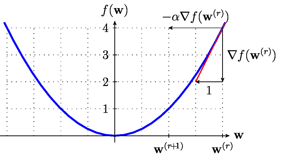
To implement the GD step \eqref{equ_def_GD_step} we need to choose a useful learning rate [math]\lrate[/math]. Moreover, executing the GD step \eqref{equ_def_GD_step} requires to compute the gradient [math]\nabla f(\weights^{(\itercntr)})[/math]. Both tasks can be computationally challenging as discussed in Section Choosing the Learning Rate and Stochastic GD . For the objective function \eqref{equ_obj_emp_risk_GD} obtained in linear regression and logistic regression, we can obtain closed-form expressions for the gradient [math]\nabla f(\weights)[/math] (see Section GD for Linear Regression and GD for Logistic Regression ).

In general, we do not have closed-form expressions for the gradient of the objective function \eqref{equ_obj_emp_risk_GD} arising from a non-linear hypothesis space. One example for such a hypothesis space is obtained from a ANN, which is used by deep learning methods (see Section Deep Learning ). The empirical success of deep learning methods might be partially attributed to the availability of an efficient algorithm for computing the gradient [math]\nabla f(\weights^{(\itercntr)})[/math]. This algorithm is known as \index{back-propagation}back-propagation .

Choosing the Learning Rate

Effect of choosing bad values for the learning rate [math]\lrate[/math] in the GD step\eqref{equ_def_GD_step}. (a) If the learning rate [math]\lrate[/math] in the GD step \eqref{equ_def_GD_step} is chosen too small, the iterations make very little progress towards the optimum or even fail to reach the optimum at all.

Effect of choosing bad values for the learning rate [math]\lrate[/math] in the GD step\eqref{equ_def_GD_step}. (b) If the learning rate [math]\lrate[/math] is chosen too large, the iterates [math]\weights^{(\itercntr)}[/math] might not converge at all (it might happen that [math]f(\weights^{(\itercntr\!+\!1)}) \gt f(\weights^{(\itercntr)})[/math]!).

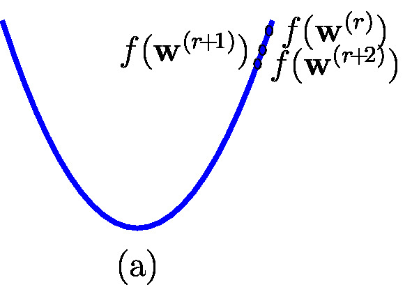
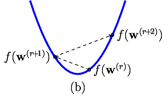
The choice of the learning rate [math]\lrate[/math] in the GD step \eqref{equ_def_GD_step} has a significant impact on the performance of Algorithm alg:gd_linreg. If we choose the learning rate [math]\lrate[/math] too large, the GD steps \eqref{equ_def_GD_step} diverge (see Figure fig_small_large_lrate-(b)) and, in turn, Algorithm alg:gd_linreg fails to deliver a satisfactory approximation of the optimal weights [math]\overline{\weights}[/math].

If we choose the learning rate [math]\lrate[/math] too small (see Figure fig_small_large_lrate-(a)), the updates \eqref{equ_def_GD_step} make only very little progress towards approximating the optimal parameter vector [math]\overline{\weights}[/math]. In applications that require real-time processing of data streams, it might be possible to repeat the GD steps only for a moderate number. Thus If the learning rate is chosen too small, Algorithm alg:gd_linreg will fail to deliver a good approximation within an acceptable number of iterations (runtime of Algorithm alg:gd_linreg).

Finding a (nearly) optimal choice for the learning rate [math]\lrate[/math] of GD can be a challenging task. Many sophisticated approaches for tuning the learning rate of gradient-based methods have been proposed . A detailed discussion of these approaches is beyond the scope of this book. We will instead discuss two sufficient conditions on the learning rate which guarantee the convergence of the GD iterations to the optimum of a smooth and convex objective function \eqref{equ_obj_emp_risk_GD}.

The first condition applies to an objective function that is [math]\beta[/math]-smooth (see \eqref{equ_def_beta_smooth}) with known constant [math]\beta[/math] (not necessarily the smallest constant such that \eqref{equ_def_beta_smooth} holds). Then, the iterates [math]\weights^{(\itercntr)}[/math] generated by the GD step \eqref{equ_def_GD_step} with a learning rate

[[math]] \begin{equation} \label{equ_suff_cond_lrate_beta} \lrate \lt 2/\beta, \end{equation} [[/math]]

satisfy

[[math]] \begin{equation} \label{equ_convergence_rate_inverse_k-GD} f \big( \weights^{(\itercntr)} \big) - \bar{f} \leq \frac{2(f \big( \weights^{(0)} \big) - \bar{f}) \sqeuclnorm{\weights^{(0)} -\overline{\weights}}}{2\sqeuclnorm{ \weights^{(0)} - \overline{\weights}}+\itercntr(f \big( \weights^{(0)} \big) -\bar{f}) \lrate(2-\beta\lrate)}. \end{equation} [[/math]]

The bound \eqref{equ_convergence_rate_inverse_k-GD} not only tells us that GD iterates converge to an optimal parameter vector but also characterize the convergence speed or rate. The sub-optimality [math]f \big( \weights^{(\itercntr)} \big) - \min_{\weights} f(\weights)[/math] in terms of objective function value decreases inversely (like “[math]1/\itercntr[/math]”) with the number [math]\itercntr[/math] of GD steps \eqref{equ_def_GD_step}. Convergence bounds like \eqref{equ_convergence_rate_inverse_k-GD} can be used to specify a stopping criterion, i.e., to determine the number of GD steps to be computed (see Section When To Stop? ).

The condition \eqref{equ_suff_cond_lrate_beta} and the bound \eqref{equ_convergence_rate_inverse_k-GD} is only useful if we can verify [math]\beta[/math] smoothness \eqref{equ_def_beta_smooth} assumption for a reasonable constant [math]\beta[/math]. Verifying \eqref{equ_convergence_rate_inverse_k-GD} only for a very large [math]\beta[/math] results in the bound \eqref{equ_convergence_rate_inverse_k-GD} being too loose (pessimistic). When we use a loose bound \eqref{equ_convergence_rate_inverse_k-GD} to determine the number of GD steps, we might compute an unnecessary large number of GD steps \eqref{equ_def_GD_step}.

One elegant approach to verify if a differentiable function [math]f(\weights)[/math] is [math]\beta[/math] smooth \eqref{equ_def_beta_smooth} is via the Hessian matrix [math] \nabla^{2} f(\weights) \in \mathbb{R}^{\featuredim \times \featuredim}[/math] if it exists. The entries of this Hessian matrix are the second-order partial derivatives [math]\frac{\partial f(\weights)}{\partial \weight_{\featureidx} \partial \weight_{\featureidx'}}[/math] of the function [math]f(\weights)[/math].

Consider an objective function [math]f(\weights)[/math] \eqref{equ_obj_emp_risk_GD} that is convex and twice-differentiable with positive semi-definite (psd) Hessian [math]\nabla^{2} f(\weights)[/math]. If the maximum eigenvalue [math]\eigval{\rm max} \big( \nabla^{2} f(\weights) \big)[/math] of the Hessian is upper bounded uniformly (for all [math]\weights[/math]) by the constant [math]\beta\gt0[/math], then [math]f(\weights)[/math] is [math]\beta[/math] smooth \eqref{equ_def_beta_smooth} . This implies, in turn via \eqref{equ_suff_cond_lrate_beta}, the sufficient condition

[[math]] \begin{equation} \label{equ_GD_conv_guarantee} \lrate \leq \frac{2}{\eigval{\rm max} \big( \nabla^{2} f(\weights) \big) }\mbox{ for all } \vw \in \mathbb{R}^{\featuredim} \end{equation} [[/math]]

for the GD learning rate such that the GD steps converge to the minimum of the objective function [math]f(\weights)[/math].

It is important to note that the condition \eqref{equ_GD_conv_guarantee} guarantees convergence of the GD steps for any possible initialization [math]\weights^{(0)}[/math]. Note that the usefulness of the condition \eqref{equ_GD_conv_guarantee} depends on the difficulty of computing the Hessian matrix [math]\nabla^{2} f(\weights)[/math]. Section GD for Linear Regression and Section GD for Logistic Regression will present closed-form expressions for the Hessian of the objective function \eqref{equ_obj_emp_risk_GD} obtained for linear regression and logistic regression. These closed-form expressions involve the feature vectors and labels of the data points in the training set [math]\dataset = \big\{ \big(\featurevec^{(1)},\truelabel^{(1)} \big),\ldots,\big(\featurevec^{(\samplesize)},\truelabel^{(\samplesize)} \big) \big\}[/math] used in \eqref{equ_obj_emp_risk_GD}.

While it might be computationally challenging to determine the maximum (in absolute value) eigenvalue [math]\eigval{\rm max} \big( \nabla^{2} f(\weights) \big)[/math] for arbitrary [math]\weights[/math], it might still be feasible to find an upper bound [math]U[/math] for it. If we know such an upper bound [math]U \geq \eigval{\rm max} \big( \nabla^{2} f(\weights) \big)[/math] (valid for all [math]\weights \in \mathbb{R}^{\featuredim}[/math]), the learning rate [math]\lrate =1/U[/math] still ensures convergence of the GD steps \eqref{equ_def_GD_step}.

Up to know we have assumed a fixed (constant) learning rate [math]\lrate[/math] that is used for each repetition of the GD steps \eqref{equ_def_GD_step}. However, it might be useful to vary or adjust the learning rate as the GD steps \eqref{equ_def_GD_step} proceed. Thus, we might use a different learning rate [math]\lrate_{\itercntr}[/math] for each iteration [math]\itercntr[/math] of \eqref{equ_def_GD_step}. Such a varying learning rate is useful for a variant of GD that uses stochastic approximation (see Section Stochastic GD ). However, we might use a varying learning rate also to avoid the burden of verifying [math]\beta[/math] smoothness \eqref{equ_def_beta_smooth} with a tight (small) [math]\beta[/math]. The GD steps \eqref{equ_def_GD_step} with the learning rate [math]\lrate_{\itercntr} \defeq 1/\itercntr[/math] converge to the optimal parameter vector [math]\overline{\weights}[/math] as long as we can ensure a bounded gradient [math]\| \nabla f(\weights) \| \leq U[/math] for a sufficiently large neighbourhood of [math]\overline{\weights}[/math] .

When To Stop?

One main challenge in the successful application of GD is to decide when to stop iterating (or repeating) the GD step \eqref{equ_def_GD_step}. Maybe the most simple approach is to monitor the decrease in the objective function [math]f(\weights^{(\itercntr)})[/math] and to stop if the decrease [math]f(\weights^{(\itercntr-1)})-f(\weights^{(\itercntr)})[/math] falls below a threshold. However, the ultimate goal of a ML method is not to minimize the objective function [math]f(\weights)[/math] in \eqref{equ_obj_emp_risk_GD}. Indeed, the objective function represents the average loss of a hypothesis [math]h^{(\weights)}[/math] incurred on a training set. However, the ultimate goal of a ML method is to learn a parameter vector [math]\weights[/math] such that the resulting hypothesis accurately predicts any data point, including those outside the training set.

We will see in Chapter Model Validation and Selection how to use validation techniques to probe a hypothesis outside the training set. These validation techniques provide a validation error [math]\tilde{f}(\weights)[/math] that estimates the average loss of a hypothesis with parameter vector [math]\weights[/math]. Early stopping techniques monitor the validation error [math]\tilde{f}(\weights^{(\itercntr)})[/math] as the GD iterations [math]\itercntr[/math] proceed to decide when to stop iterating.

Another possible stopping criterion is to use a fixed number of iterations or GD steps. This fixed number of iterations can be chosen based on convergence bounds such as \eqref{equ_convergence_rate_inverse_k-GD} in order to guarantee a prescribed sub-optimality of the final iterate [math]\weights^{(\itercntr)}[/math]. A slightly more convenient convergence bound can be obtained from \eqref{equ_convergence_rate_inverse_k-GD} when using the the learning rate [math]\lrate = 1/\beta[/math] in the GD step \eqref{equ_def_GD_step} ,

[[math]] \begin{equation} f \big( \weights^{(\itercntr)} \big) -\bar{f} \leq \frac{2\beta \sqeuclnorm{\weights^{(0)} -\overline{\weights}}}{\itercntr} \mbox{ for } \itercntr=1,2,\ldots. \end{equation} [[/math]]

GD for Linear Regression

We now present a gradient based method for learning the parameter vector for a linear hypothesis (see equ_lin_hypospace)

[[math]] \begin{equation} \label{equ_def_lin_pred_GD} h^{(\weights)}(\featurevec) = \weights^{T} \featurevec. \end{equation} [[/math]]

The ERM principle tells us to choose the parameter vector [math]\weights[/math] in \eqref{equ_def_lin_pred_GD} by minimizing the average squared error loss

[[math]] \begin{equation} \label{equ_def_cost_linreg} \emperror(h^{(\weights)}| \dataset) \stackrel{\eqref{eq_def_ERM_weight}}{=} (1/\samplesize) \sum_{\sampleidx=1}^{\samplesize} (\truelabel^{(\sampleidx)} - \weights^{T} \featurevec^{(\sampleidx)})^{2}. \end{equation} [[/math]]

The average squared error loss \eqref{equ_def_cost_linreg} is computed by applying the predictor [math]h^{(\weights)}(\featurevec)[/math] to labeled data points in a training set [math]\dataset=\{ (\featurevec^{(\sampleidx)}, \truelabel^{(\sampleidx)}) \}_{\sampleidx=1}^{\samplesize}[/math]. An optimal parameter vector [math]\overline{\weights}[/math] for \eqref{equ_def_lin_pred_GD} is obtained as

[[math]] \begin{equation} \label{equ_smooth_problem_linreg} \overline{\weights} = \argmin_{\weights \in \mathbb{R}^{\featuredim}} f(\weights) \mbox{ with } f(\weights) = (1/\samplesize) \sum_{\sampleidx=1}^{\samplesize} \big(\truelabel^{(\sampleidx)} - \weights^{T} \featurevec^{(\sampleidx)}\big)^{2}. \end{equation} [[/math]]

The objective function [math]f(\weights)[/math] in \eqref{equ_smooth_problem_linreg} is convex and smooth. We can therefore use GD \eqref{equ_def_GD_step} to solve \eqref{equ_smooth_problem_linreg} iteratively, i.e., by constructing a sequence of parameter vectors that converge to an optimal parameter vector [math]\overline{\weights}[/math]. To implement GD, we need to compute the gradient [math]\nabla f(\weights)[/math].

The gradient of the objective function in \eqref{equ_smooth_problem_linreg} is given by

[[math]] \begin{equation} \label{equ_gradient_linear_regression} \nabla f(\weights) = -(2/\samplesize) \sum_{\sampleidx=1}^{\samplesize} \big(\truelabel^{(\sampleidx)} - \weights^{T} \featurevec^{(\sampleidx)} \big) \featurevec^{(\sampleidx)}. \end{equation} [[/math]]

By inserting \eqref{equ_gradient_linear_regression} into the basic GD iteration \eqref{equ_def_GD_step}, we obtain Algorithm alg:gd_linreg.

Linear regression via GD

Input: dataset [math]\dataset=\{ (\featurevec^{(\sampleidx)}, \truelabel^{(\sampleidx)}) \}_{\sampleidx=1}^{\samplesize}[/math] ; learning rate [math]\lrate \gt0[/math].

Initialize: set [math]\weights^{(0)}\!\defeq\!\mathbf{0}[/math]; set iteration counter [math]\itercntr\!\defeq\!0[/math]

• repeat
• [math]\itercntr \defeq \itercntr +1[/math] (increase iteration counter)
• [math]\weights^{(\itercntr)} \defeq \weights^{(\itercntr\!-\!1)} + \lrate (2/\samplesize) \sum_{\sampleidx=1}^{\samplesize} \big(\truelabel^{(\sampleidx)} - \big(\weights^{(\itercntr\!-\!1)}\big)^{T} \featurevec^{(\sampleidx)}\big) \featurevec^{(\sampleidx)}[/math] (do a GD step \eqref{equ_def_GD_step})
• until stopping criterion met

Output: [math]\weights^{(\itercntr)}[/math] (which approximates [math]\overline{\weights}[/math] in \eqref{equ_smooth_problem_linreg})

Let us have a closer look on the update in step [math]3[/math] of Algorithm alg:gd_linreg, which is

[[math]] \begin{equation} \label{equ_update_gd_linreg} \weights^{(\itercntr)} \defeq \weights^{(\itercntr\!-\!1)} + \lrate (2/\samplesize) \sum_{\sampleidx=1}^{\samplesize} \big(\truelabel^{(\sampleidx)} - \big(\weights^{(\itercntr\!-\!1)})^{T} \featurevec^{(\sampleidx)} \big) \featurevec^{(\sampleidx)}. \end{equation} [[/math]]

The update \eqref{equ_update_gd_linreg} has an appealing form as it amounts to correcting the previous guess (or approximation) [math]\weights^{(\itercntr\!-\!1)}[/math] for the optimal parameter vector [math]\overline{\weights}[/math] by the correction term

[[math]] \begin{equation} \label{equ_corr_term_linreg} (2\lrate/\samplesize) \sum_{\sampleidx=1}^{\samplesize} \underbrace{(\truelabel^{(\sampleidx)} - \big(\weights^{(\itercntr\!-\!1)})^{T} \featurevec^{(\sampleidx)})}_{e^{(\sampleidx)}} \featurevec^{(\sampleidx)}. \end{equation} [[/math]]

The correction term \eqref{equ_corr_term_linreg} is a weighted average of the feature vectors [math]\featurevec^{(\sampleidx)}[/math] using weights [math](2\lrate/\samplesize) \cdot e^{(\sampleidx)}[/math]. These weights consist of the global factor [math](2\lrate/\samplesize)[/math] (that applies equally to all feature vectors [math]\featurevec^{(\sampleidx)}[/math]) and a sample-specific factor [math]e^{(\sampleidx)} = (\truelabel^{(\sampleidx)} - \big(\weights^{(\itercntr\!-\!1)})^{T} \featurevec^{(\sampleidx)})[/math], which is the prediction (approximation) error obtained by the linear predictor [math]h^{(\weights^{(\itercntr\!-\!1)})}(\featurevec^{(\sampleidx)}) = \big(\weights^{(\itercntr\!-\!1)})^{T} \featurevec^{(\sampleidx)}[/math] when predicting the label [math]\truelabel^{(\sampleidx)}[/math] from the features [math]\featurevec^{(\sampleidx)}[/math].

We can interpret the GD step \eqref{equ_update_gd_linreg} as an instance of “learning by trial and error”. Indeed, the GD step amounts to first “trying out” (trial) the predictor [math]h(\featurevec^{(\sampleidx)}) = \big(\weights^{(\itercntr\!-\!1)})^{T}\featurevec^{(\sampleidx)}[/math]. The predicted values are then used to correct the weight vector [math]\weights^{(\itercntr\!-\!1)}[/math] according to the error [math]e^{(\sampleidx)} = \truelabel^{(\sampleidx)} - \big(\weights^{(\itercntr\!-\!1)})^{T} \featurevec^{(\sampleidx)}[/math].

The choice of the learning rate [math]\lrate[/math] used for Algorithm alg:gd_linreg can be based on the condition \eqref{equ_GD_conv_guarantee} with the Hessian [math]\nabla^{2} f(\weights)[/math] of the objective function [math]f(\weights)[/math] underlying linear regression (see \eqref{equ_smooth_problem_linreg}). This Hessian is given explicitly as

[[math]] \begin{equation} \label{equ_hessian_linreg} \nabla^{2} f(\weights) = (1/\samplesize) \featuremtx^{T} \featuremtx, \end{equation} [[/math]]

with the feature matrix [math]\featuremtx=\big(\featurevec^{(1)},\ldots,\featurevec^{(\samplesize)}\big)^{T} \in \mathbb{R}^{\samplesize \times \featuredim}[/math] (see feature matrix ). Note that the Hessian \eqref{equ_hessian_linreg} does not depend on the parameter vector [math]\weights[/math].

Comparing \eqref{equ_hessian_linreg} with \eqref{equ_GD_conv_guarantee}, one particular strategy for choosing the learning rate in Algorithm alg:gd_linreg is to (i) compute the matrix product [math] \featuremtx^{T} \featuremtx[/math], (ii) compute the maximum eigenvalue [math]\eigval{\rm max}\big( (1/\samplesize) \featuremtx^{T} \featuremtx \big)[/math] of this product and (iii) set the learning rate to [math]\lrate =1/\eigval{\rm max} \big( (1/\samplesize) \featuremtx^{T} \featuremtx \big)[/math].

While it might be challenging to compute the maximum eigenvalue [math]\eigval{\rm max} \big( (1/\samplesize) \featuremtx^{T} \featuremtx \big)[/math], it might be easier to find an upper bound [math]U[/math] for it.

Given such an upper bound [math]U \geq \eigval{\rm max} \big( (1/\samplesize) \featuremtx^{T} \featuremtx \big)[/math], the learning rate [math]\lrate =1/U[/math] still ensures convergence of the GD steps. Consider a dataset [math]\{(\featurevec^{(\sampleidx)},\truelabel^{(\sampleidx)})\}_{\sampleidx=1}^{\samplesize}[/math] with normalized features, i.e., [math]\| \featurevec^{(\sampleidx)}\| = 1[/math] for all [math]\sampleidx =1,\ldots,\samplesize[/math]. This implies, in turn, the upper bound [math]U= 1[/math], i.e., [math] 1 \geq \lambda_{\rm max} \big( (1/\samplesize) \featuremtx^{T} \featuremtx \big)[/math]. We can then ensure convergence of the iterates [math]\weights^{(\itercntr)}[/math] (see \eqref{equ_update_gd_linreg}) by choosing the learning rate [math]\lrate =1[/math].

Time-Data Tradeoffs. The number of GD steps required by Algorithm alg:gd_linreg to ensure a prescribed sub-optimality depends crucially on the condition number of [math]\featuremtx^{T} \featuremtx[/math]. What can we say about the condition number? In general, we have not control over this quantity as the matrix [math]\featuremtx[/math] consists of the feature vectors of arbitrary data points. However, it is often useful to model the feature vectors as realizations of independent and identically distributed (iid) random vectors. It is then possible to bound the probability of the feature matrix having a sufficiently small condition number. These bounds can then be used to choose the step-size such that convergence is guaranteed with sufficiently large probability. The usefulness of these bounds typically depends on the ratio [math]\featurelen/\samplesize[/math]. For increasing sample-size, these bounds allow to use larger step-sizes and, in turn, result in faster convergence of GD algorithm. Thus, we obtain a trade-off between the runtime of Algorithm alg:gd_linreg and the number of data points that we feed into it .

GD for Logistic Regression

Logistic regression learns a linear hypothesis [math]h^{(\weights)}[/math] that is used to classify data points by predicting their binary label. The quality of such a linear classifier is measured by the logistic loss. The ERM principle suggest to learn the parameter vector [math]\weights[/math] by minimizing the average logistic loss obtained for a training set [math]\dataset= \{ (\featurevec^{(\sampleidx)}, \truelabel^{(\sampleidx)}) \}_{\sampleidx=1}^{\samplesize}[/math]. The training set consists of data points with features [math]\featurevec^{(\sampleidx)} \in \mathbb{R}^{\featuredim}[/math] and binary labels [math]\truelabel^{(\sampleidx)} \in \{-1,1\}[/math].

We can rewrite ERM for logistic regression as the optimization problem

[[math]] \begin{align} \overline{\weights}& = \argmin_{\weights \in \mathbb{R}^{\featuredim}} f(\weights) \nonumber \\ \mbox{ with } f(\weights) & = \label{equ_smooth_problem_logeg}(1/\samplesize) \sum_{\sampleidx=1}^{\samplesize} \log\big( 1\!+\!\exp \big( - \truelabel^{(\sampleidx)} \weights^{T} \featurevec^{(\sampleidx)} \big)\big). \end{align} [[/math]]

The objective function [math]f(\weights)[/math] is differentiable and therefore we can use GD \eqref{equ_def_GD_step} to solve \eqref{equ_smooth_problem_logeg}. We can write down the gradient of the objective function in \eqref{equ_smooth_problem_logeg} in closed-form as

[[math]] \begin{equation} \label{equ_gradient_logistic_regression} \nabla f(\weights) = (1/\samplesize) \sum_{\sampleidx=1}^{\samplesize} \frac{-\truelabel^{(\sampleidx)}}{1 + \exp ( \truelabel^{(\sampleidx)} \weights^{T} \featurevec^{(\sampleidx)})} \featurevec^{(\sampleidx)}. \end{equation} [[/math]]

Inserting \eqref{equ_gradient_logistic_regression} into the GD step \eqref{equ_def_GD_step} yields Algorithm alg:gd_logreg.

Logistic regression via GD

Input: labeled dataset [math]\dataset=\{ (\featurevec^{(\sampleidx)}, \truelabel^{(\sampleidx)}) \}_{\sampleidx=1}^{\samplesize}[/math] containing feature vectors [math]\featurevec^{(\sampleidx)} \in \mathbb{R}^{\featuredim}[/math] and labels [math]\truelabel^{(\sampleidx)} \in \mathbb{R}[/math]; GD learning rate [math]\lrate \gt0[/math].

Initialize: set [math]\weights^{(0)}\!\defeq\!\mathbf{0}[/math]; set iteration counter [math]\itercntr\!\defeq\!0[/math]

• repeat
• [math]\itercntr\!\defeq\! \itercntr\!+\!1[/math] (increase iteration counter)
• [math]\weights^{(\itercntr)} \defeq \weights^{(\itercntr\!-\!1)}\!+\!\lrate (1/\samplesize) \sum_{\sampleidx=1}^{\samplesize} \frac{\truelabel^{(\sampleidx)}}{1\!+\!\exp \big( \truelabel^{(\sampleidx)} \big(\weights^{(\itercntr\!-\!1)}\big)^{T} \featurevec^{(\sampleidx)}\big)} \featurevec^{(\sampleidx)}[/math] (do a GD step \eqref{equ_def_GD_step})
• until stopping criterion met

Output: [math]\weights^{(\itercntr)}[/math], which approximates a solution [math]\overline{\weights}[/math] of \eqref{equ_smooth_problem_logeg})

Let us have a closer look on the update in step equ_step_updat_logreg_GD of Algorithm alg:gd_logreg. This step amounts to computing

[[math]] \begin{equation} \label{equ_update_logreg_GD} \weights^{(\itercntr)} \defeq \weights^{(\itercntr\!-\!1)} + \lrate (1/\samplesize) \sum_{\sampleidx=1}^{\samplesize} \frac{\truelabel^{(\sampleidx)}}{1 + \exp \big( \truelabel^{(\sampleidx)} \big( \vw^{(\itercntr\!-\!1)} \big)^{T} \featurevec^{(\sampleidx)}\big)} \featurevec^{(\sampleidx)}. \end{equation} [[/math]]

Similar to the GD step \eqref{equ_update_gd_linreg} for linear regression, also the GD step \eqref{equ_update_logreg_GD} for logistic regression can be interpreted as an implementation of the trial-and-error principle. Indeed, \eqref{equ_update_logreg_GD} corrects the previous guess (or approximation) [math]\weights^{(\itercntr\!-\!1)}[/math] for the optimal parameter vector [math]\overline{\weights}[/math] by the correction term

[[math]] \begin{equation} \label{equ_correction_logreg_GD} (\lrate/\samplesize) \sum_{\sampleidx=1}^{\samplesize} \underbrace{ \frac{\truelabel^{(\sampleidx)}}{1 + \exp ( \truelabel^{(\sampleidx)} \weights^{T} \featurevec^{(\sampleidx)})}}_{e^{(\sampleidx)}} \featurevec^{(\sampleidx)}. \end{equation} [[/math]]

The correction term \eqref{equ_correction_logreg_GD} is a weighted average of the feature vectors [math]\featurevec^{(\sampleidx)}[/math]. The feature vector [math]\featurevec^{(\sampleidx)}[/math] is weighted by the factor [math](\lrate/\samplesize) \cdot e^{(\sampleidx)}[/math]. These weighting factors are a product of the global factor [math](\lrate/\samplesize)[/math] that applies equally to all feature vectors [math]\featurevec^{(\sampleidx)}[/math]. The global factor is multiplied by a data point-specific factor [math]e^{(\sampleidx)} = \frac{\truelabel^{(\sampleidx)}}{1 + \exp ( \truelabel^{(\sampleidx)} \weights^{T} \featurevec^{(\sampleidx)})}[/math], which quantifies the error of the classifier [math]h^{(\weights^{(\itercntr\!-\!1)})}(\featurevec^{(\sampleidx)}) = \big(\weights^{(\itercntr\!-\!1)})^{T} \featurevec^{(\sampleidx)}[/math] for a single data point with true label [math]\truelabel^{(\sampleidx)} \in \{-1,1\}[/math] and features [math]\featurevec^{(\sampleidx)} \in \mathbb{R}^{\featuredim}[/math].

We can use the sufficient condition \eqref{equ_GD_conv_guarantee} for the convergence of GD steps to guide the choice of the learning rate [math]\lrate[/math] in Algorithm alg:gd_logreg. To apply condition \eqref{equ_GD_conv_guarantee}, we need to determine the Hessian [math]\nabla^{2} f(\weights)[/math] matrix of the objective function [math]f(\weights)[/math] underlying logistic regression (see \eqref{equ_smooth_problem_logeg}). Some basic calculus reveals (see )

[[math]] \begin{equation} \label{equ_hessian_logreg} \nabla^{2} f(\weights) = (1/\samplesize) \mX^{T} \mD \featuremtx. \end{equation} [[/math]]

Here, we used the feature matrix [math]\featuremtx=\big(\featurevec^{(1)},\ldots,\featurevec^{(\samplesize)}\big)^{T} \in \mathbb{R}^{\samplesize \times \featuredim}[/math] (see feature matrix ) and the diagonal matrix [math]\mD = {\rm diag} \{d_{1},\ldots,d_{\samplesize}\} \in \mathbb{R}^{\samplesize \times \samplesize}[/math] with diagonal elements

[[math]] \begin{equation} d_{\sampleidx} = \frac{1}{1+\exp(-\weights^{T} \featurevec^{(\sampleidx)})} \bigg(1- \frac{1}{1+\exp(-\weights^{T} \featurevec^{(\sampleidx)})} \bigg). \label{equ_diag_entries_log_reg} \end{equation} [[/math]]

We highlight that, in contrast to the Hessian \eqref{equ_hessian_linreg} of the objective function arising in linear regression, the Hessian \eqref{equ_hessian_logreg} of logistic regression varies with the parameter vector [math]\weights[/math]. This makes the analysis of Algorithm alg:gd_logreg and the optimal choice for the learning rate [math]\lrate[/math] more difficult compared to Algorithm alg:gd_linreg. At least, we can ensure convergence of \eqref{equ_update_logreg_GD} (towards a solution of \eqref{equ_smooth_problem_logeg}) for the learning rate [math]\lrate=1[/math] if we normalize feature vectors such that [math]\| \featurevec^{(\sampleidx)} \|=1[/math]. This follows from the fact the diagonal entries \eqref{equ_diag_entries_log_reg} take values in the interval [math][0,1][/math].

Data Normalization

The number of GD steps \eqref{equ_def_GD_step} required to reach the minimum (within a prescribed accuracy) of the objective function depends crucially on the condition number

[[math]] \begin{equation} \label{equ_def_condition_number} \kappa( \featuremtx^{T} \featuremtx) \defeq \eigval{\rm max}/\eigval{\rm min}. \end{equation} [[/math]]

Here, we use the largest and smallest eigenvalue of the matrix [math]\featuremtx^{T} \featuremtx[/math], denoted as [math] \eigval{\rm max}[/math] and [math]\eigval{\rm min}[/math], respectively. The condition number \eqref{equ_def_condition_number} is only well-defined if the columns of the feature matrix [math]\featuremtx[/math] (which are the feature vectors [math]\featurevec^{(\sampleidx)}[/math]), are linearly independent. In this case the condition number is lower bounded as [math]1 \leq \kappa( \featuremtx^{T} \featuremtx)[/math].

It can be shown that the GD steps \eqref{equ_def_GD_step} converge faster for smaller condition number [math]\kappa( \featuremtx^{T} \featuremtx)[/math] . Thus, GD will be faster for datasets with a feature matrix [math]\featuremtx[/math] such that [math]\kappa( \featuremtx^{T} \featuremtx) \approx 1[/math]. It is therefore often beneficial to pre-process the feature vectors using a normalization (or standardization) procedure as detailed in Algorithm alg_reshaping.

“Data Normalization”

Input: labeled dataset [math]\dataset = \{(\featurevec^{(\sampleidx)},y^{(\sampleidx)})\}_{\sampleidx=1}^{\samplesize}[/math]

• remove sample means [math]\widehat{\featurevec}=(1/\samplesize) \sum_{\sampleidx=1}^{\samplesize} \featurevec^{(\sampleidx)}[/math] from features, i.e.,
  [[math]] \begin{equation} \nonumber \featurevec^{(\sampleidx)} \defeq \featurevec^{(\sampleidx)} - \widehat{\featurevec} \mbox{ for } \sampleidx=1,\ldots,\samplesize \end{equation} [[/math]]
• normalise features to have unit variance,
  [[math]] \begin{equation} \nonumber \hat{\feature}^{(\sampleidx)}_{\featureidx} \defeq \feature^{(\sampleidx)}_{\featureidx}/ \hat{\sigma} \mbox{ for } \featureidx=1,\ldots,\featuredim \mbox{ and } \sampleidx=1,\ldots,\samplesize \end{equation} [[/math]]
  with the empirical (sample) variance [math]\hat{\sigma}_{\featureidx}^{2} =(1/\samplesize) \sum_{\sampleidx=1}^{\samplesize} \big( \feature^{(\sampleidx)}_{\featureidx} \big)^{2}[/math]

Output: normalized feature vectors [math]\{\hat{\featurevec}^{(\sampleidx)}\}_{\sampleidx=1}^{\samplesize}[/math]

Algorithm alg_reshaping transforms the original feature vectors [math]\featurevec^{(\sampleidx)}[/math] into new feature vectors [math]\widehat{\featurevec}^{(\sampleidx)}[/math] such that the new feature matrix [math]\widehat{\featuremtx} = (\widehat{\featurevec}^{(1)},\ldots,\widehat{\featurevec}^{(\samplesize)})^{T}[/math] is better conditioned than the original feature matrix, i.e., [math]\kappa( \widehat{\featuremtx}^{T} \widehat{\featuremtx}) \lt \kappa( \featuremtx^{T} \featuremtx)[/math].

Stochastic GD

Consider the GD steps \eqref{equ_def_GD_step} for minimizing the empirical risk \eqref{equ_obj_emp_risk_GD}. The gradient [math]\nabla f(\weights)[/math] of the objective function \eqref{equ_obj_emp_risk_GD} has a particular structure. Indeed, this gradient is a sum

[[math]] \begin{equation} \label{eq_gradient_sum} \nabla f(\weights) = (1/\samplesize) \sum_{\sampleidx=1}^{\samplesize} \nabla f_{\sampleidx}(\vw) \mbox{ with } f_{\sampleidx}(\weights) \defeq \loss{(\featurevec^{(\sampleidx)},\truelabel^{(\sampleidx)})}{h^{(\weights)}}. \end{equation} [[/math]]

Each component of the sum \eqref{eq_gradient_sum} corresponds to one particular data points [math](\featurevec^{(\sampleidx)},\truelabel^{(\sampleidx)})[/math], for [math]\sampleidx=1,\ldots,\samplesize[/math]. We need to compute a sum of the form \eqref{eq_gradient_sum} for each new GD step \eqref{equ_def_GD_step}.

Computing the sum in \eqref{eq_gradient_sum} can be computationally challenging for at least two reasons. First, computing the sum is challenging for very large datasets with [math]\samplesize[/math] in the order of billions. Second, for datasets which are stored in different data centres located all over the world, the summation would require a huge amount of network resources. Moreover, the finite transmission rate of communication networks limits the rate by which the GD steps \eqref{equ_def_GD_step} can be executed.

The idea of stochastic gradient descent (SGD) is to replace the exact gradient [math]\nabla f(\weights)[/math] \eqref{eq_gradient_sum} by an approximation that is easier to compute than a direct evaluation of \eqref{eq_gradient_sum}. The word “stochastic” in the name SGD hints already at the use of a stochastic approximation [math]\noisygrad(\weights) \approx \nabla f(\weights)[/math]. It turns out that using a gradient approximation [math]\noisygrad(\weights)[/math] can result in significant savings in computational complexity while incurring a graceful degradation in the overall optimization accuracy. The optimization accuracy (distance to minimum of [math]f(\weights)[/math]) depends crucially on the “gradient noise”

[[math]] \begin{equation} \label{equ_def_gradient_noise_generic} \varepsilon \defeq \nabla f(\weights)- \noisygrad(\weights). \end{equation} [[/math]]

The elementary step of most SGD methods is obtained from the GD step \eqref{equ_def_GD_step} by replacing the exact gradient [math]\nabla f(\weights)[/math] with some stochastic approximation [math]\noisygrad(\weights)[/math],

[[math]] \begin{equation} \label{equ_SGD_update} \weights^{(\itercntr\!+\!1)} = \weights^{(\itercntr)} - \lrate_{\itercntr} \noisygrad \big( \weights^{(\itercntr)} \big), \end{equation} [[/math]]

As the notation in \eqref{equ_SGD_update} indicates, SGD methods use a learning rate [math]\lrate_{\itercntr}[/math] that varies between different iterations.

To avoid accumulation of the gradient noise \eqref{equ_def_gradient_noise_generic} during the SGD updates \eqref{equ_SGD_update}, SGD methods typically decrease the learning rate [math]\lrate_{\itercntr}[/math] as the iterations proceed. The precise dependence of the learning rate [math]\lrate_{\itercntr}[/math] on the iteration index [math]\itercntr[/math] is referred to as a learning rate schedule . One possible choice for the learning rate schedule is [math]\lrate_{\itercntr}\!\defeq\!1/\itercntr[/math] . Exercise discusses conditions on the learning rate schedule that guarantee convergence of the updates SGD to the minimum of [math]f(\weights)[/math].

The approximate (“noisy”) gradient [math]\noisygrad(\weights)[/math] can be obtained by different randomization strategies. The most basic form of SGD constructs the gradient approximation [math]\noisygrad(\weights)[/math] by replacing the sum \eqref{eq_gradient_sum} with a randomly selected component,

[[math]] \begin{equation} \noisygrad(\weights) \defeq \nabla f_{\hat{\sampleidx}}(\weights). \end{equation} [[/math]]

The index [math]\hat{\sampleidx}[/math] is chosen randomly from the set [math]\{1,\ldots,\samplesize\}[/math]. The resulting Stochastic gradient descent (SGD) method then repeats the update

[[math]] \begin{equation} \label{equ_SGD_update_basic_form} \weights^{(\itercntr\!+\!1)} = \weights^{(\itercntr)} - \lrate \nabla f_{\hat{\sampleidx}_{\itercntr}}(\weights^{(\itercntr)}), \end{equation} [[/math]]

sufficiently often. Every update \eqref{equ_SGD_update_basic_form} uses a “fresh” randomly chosen (drawn) index [math]\hat{\sampleidx}_{\itercntr}[/math]. Formally, the indices [math]\hat{\sampleidx}_{\itercntr}[/math] are realizations of iid random variable (RV)s whose common probability distribution is the uniform distribution over the index set [math]\{1,\ldots,\samplesize\}[/math].

Note that \eqref{equ_SGD_update_basic_form} replaces the summation over the training set during the GD step \eqref{equ_def_GD_step} by randomly selecting a single component of this sum. The resulting savings in computational complexity can be significant when the training set consists of a large number of data points that might be stored in a distributed fashion (in the “cloud”). The saving in computational complexity of SGD comes at the cost of introducing a non-zero gradient noise

[[math]] \begin{align} \varepsilon_{\itercntr} & \stackrel{\eqref{equ_def_gradient_noise_generic}}{=} \nabla f( \weights^{(\itercntr)} ) - \noisygrad \big( \weights^{(\itercntr)} \big) \nonumber \\  & = \label{equ_gradient_noise_simple_form}\nabla f( \weights^{(\itercntr)} ) - \nabla f_{\hat{\sampleidx}_{\itercntr}}(\weights). \end{align} [[/math]]

Mini-Batch SGD. Let us now discuss a variant of SGD that tries to reduce the approximation error (gradient noise) \eqref{equ_gradient_noise_simple_form} arising in the SGD step \eqref{equ_SGD_update_basic_form}. The idea behind this variant, referred to as mini-batch SGD, is quite simple. Instead of using only a single randomly selected component [math]\nabla f_{\sampleidx}(\weights)[/math] (see \eqref{eq_gradient_sum}) for constructing a gradient approximation, mini-batch SGD uses several randomly chosen components.

We summarize mini-batch SGD in Algorithm alg:minibatch_gd which requires an integer batch size [math]\batchsize[/math] as input parameter. Algorithm alg:minibatch_gd repeats the SGD step \eqref{equ_SGD_update} using a gradient approximation that is constructed from a randomly selected subset [math]\batch = \{ \sampleidx_{1},\ldots,\sampleidx_{\batchsize}\}[/math] (a “batch”),

[[math]] \begin{equation} \label{equ_def_gradient_approx_mini_batch} \noisygrad \big( \weights \big) = (1/\batchsize) \sum_{\sampleidx' \in \batch} \nabla f_{\sampleidx'}(\weights). \end{equation} [[/math]]

For each new iteration of Algorithm alg:minibatch_gd, a new batch [math]\batch[/math] is generated by a random generator.

Mini-Batch SGD

Input: components [math]f_{\sampleidx}(\weights)[/math], for [math]\sampleidx=1,\ldots,\samplesize[/math] of objective function [math]f(\weights)=\sum_{\sampleidx=1}^{\samplesize} f_{\sampleidx}(\weights)[/math] ; batch size [math]\batchsize[/math]; learning rate schedule [math]\lrate_{\itercntr} \gt0[/math].

set [math]\vw^{(0)}\!\defeq\!\mathbf{0}[/math]; set iteration counter [math]\itercntr\!\defeq\!0[/math]

• repeat
• randomly select a batch [math]\batch = \{\sampleidx_{1},\ldots,\sampleidx_{\batchsize}\} \subseteq \{1,\ldots,\samplesize\}[/math] of indices that select a subset of components [math]f_{\sampleidx}[/math]
• compute an approximate gradient [math]\noisygrad \big( \weights^{(\itercntr)} \big)[/math] using \eqref{equ_def_gradient_approx_mini_batch}
• [math]\itercntr \defeq \itercntr +1[/math] (increase iteration counter)
• [math]\weights^{(\itercntr)} \defeq \weights^{(\itercntr\!-\!1)} - \lrate_{\itercntr} \noisygrad \big( \weights^{(\itercntr-1)} \big)[/math]
• until stopping criterion met

Output: [math]\weights^{(\itercntr)}[/math] (which approximates [math]\argmin_{\weights \in \mathbb{R}^{\featuredim}} f(\weights)[/math] ))

Note that Algorithm alg:minibatch_gd includes the basic SGD variant \eqref{equ_SGD_update_basic_form} as a special case for the batch size [math]\batchsize=1[/math]. Another special case is [math]\batchsize= \samplesize[/math], where the SGD step \ref{equ_sGD_step_minibtatch} in Algorithm alg:minibatch_gd becomes an ordinary GD step \eqref{equ_def_GD_step}.

Online Learning. A main motivation for the SGD step \eqref{equ_SGD_update_basic_form} is that a training set is already collected but so large that the sum in \eqref{eq_gradient_sum} is computationally intractable. Another variant of SGD is obtained for sequential (time-series) data. In particular, consider data points that are gathered sequentially, one new data point [math]\big( \featurevec^{(\timeidx)},\truelabel^{(\timeidx)} \big)[/math] at each time instant [math]\timeidx=1,2,\ldots.[/math]. With each new data point [math]\big( \featurevec^{(\timeidx)},\truelabel^{(\timeidx)} \big)[/math] we can access a new component [math]f_{\timeidx}(\weights) = \loss{(\featurevec^{(\timeidx)},\truelabel^{(\timeidx)})}{h^{(\weights)}}[/math] (see \eqref{equ_obj_emp_risk_GD}). For sequential data, we can use a slight modification of the SGD step \eqref{equ_SGD_update} to obtain an online learning method (see Section Online Learning ). This online variant of SGD computes, at each time instant [math]\timeidx[/math],

[[math]] \begin{equation} \label{equ_SGD_update_timeiedx} \weights^{(\timeidx)} \defeq \weights^{(\timeidx\!-\!1)} - \lrate_{\timeidx} \nabla f_{\timeidx}(\weights^{(\timeidx\!-\!1)}). \end{equation} [[/math]]

Advanced Gradient-Based Methods

The main idea underlying GD and SGD is to approximate the objective function \eqref{equ_obj_emp_risk_GD} locally around a current guess or approximation [math]\weights^{(\itercntr)}[/math] for the optimal weights. This local approximation is a tangent hyperplane whose normal vector is determined by the gradient [math]\nabla f (\weights^{(\itercntr)}[/math]. We then obtain an updated (improved) approximation by minimizing this local approximation, i.e., by doing a GD step \eqref{equ_def_GD_step}.

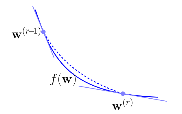
The idea of advanced gradient methods is to exploit the information provided by the gradients [math]\nabla f\big(\weights^{(\itercntr')}\big)[/math] at previous iterations [math]\itercntr'=1,\ldots,\itercntr[/math], to build an improved local approximation of [math]f(\weights)[/math] around a current iterate [math]\weights^{(\itercntr)}[/math]. Figure fig_improved_local_approx indicates such an improved local approximation of [math]f(\weights)[/math] which is non-linear (e.g., quadratic). These improved local approximations can be used to adapt the learning rate during the GD steps \eqref{equ_def_GD_step}.

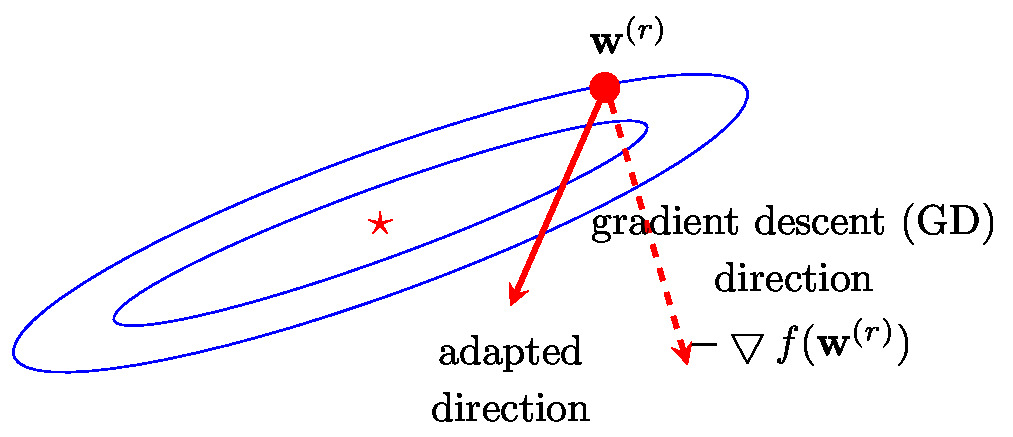
Advanced gradient-based methods use improved local approximations to modify the gradient [math]\nabla f\big(\weights^{(\itercntr')}\big)[/math] to obtain an improved update direction. Figure fig_improved_local_approx_better_directions depicts the contours of an objective function [math]f(\weights)[/math] for which the gradient [math]\nabla f\big(\weights^{(\itercntr)}\big)[/math] points only weakly towards the optimal parameter vector [math]\overline{\weights}[/math] (minimizer of [math]f(\weights)[/math]). The gradient history [math]\nabla f\big(\weights^{(\itercntr')}\big)[/math], for[math]\itercntr'=1,\ldots,\itercntr[/math], allows to detect such an unfavourable geometry of the objective function. Moreover, the gradient history can be used to “correct” the update direction [math]\nabla f\big(\weights^{(\itercntr)}\big)[/math] to obtain an improved update direction towards the optimum parameter vector [math]\overline{\weights}[/math].

Advanced gradient-based methods use the gradients at previous iterations to construct an improved (non-linear) local approximation (dashed) of the objective function [math]f(\weights)[/math] (solid).

Advanced gradient-based methods use improved (non-linear) local approximations of the objective function [math]f(\weights)[/math] to “nudge” the update direction towards the optimal parameter vector [math]\overline{\weights}[/math]. The update direction of plain vanilla GD \eqref{equ_def_GD_step} is the negative gradient [math]-\nabla f\big( \weights^{(\itercntr)}\big)[/math]. For some objective functions the negative gradient might be only weakly correlated with the straight direction from [math]\weights^{(\itercntr)}[/math] towards the optimal parameter vector ([math]\star[/math]).

General References

Jung, Alexander (2022). Machine Learning: The Basics. Signapore: Springer. doi:10.1007/978-981-16-8193-6.

Jung, Alexander (2022). "Machine Learning: The Basics". arXiv:1805.05052.

References

- 1.0 1.1 1.2 1.3 1.4 I. Goodfellow, Y. Bengio, and A. Courville. Deep Learning MIT Press, 2016
- 2.0 2.1 W. Rudin. Principles of Mathematical Analysis McGraw-Hill, New York, 3 edition, 1976
- 3.0 3.1 3.2 3.3 S. Bubeck. Convex optimization. algorithms and complexity. In Foundations and Trends in Machine Learning volume 8. Now Publishers, 2015
- 4.0 4.1 Y. Nesterov. Introductory lectures on convex optimization volume 87 of Applied Optimization. Kluwer Academic Publishers, Boston, MA, 2004. A basic course
- S. Oymak, B. Recht, and M. Soltanolkotabi. Sharp time--data tradeoffs for linear inverse problems. IEEE Transactions on Information Theory 64(6):4129--4158, June 2018
- T. Hastie, R. Tibshirani, and J. Friedman. The Elements of Statistical Learning Springer Series in Statistics. Springer, New York, NY, USA, 2001
- 7.0 7.1 A. Jung. A fixed-point of view on gradient methods for big data. Frontiers in Applied Mathematics and Statistics 3, 2017
- N. Murata. A statistical study on on-line learning. In D. Saad, editor, On-line Learning in Neural Networks pages 63--92. Cambridge University Press, New York, NY, USA, 1998