Moments

[math] \require{textmacros} \def \bbeta {\bf \beta} \def\fat#1{\mbox{\boldmath$#1$}} \def\reminder#1{\marginpar{\rule[0pt]{1mm}{11pt}}\textbf{#1}} \def\SSigma{\bf \Sigma} \def\ttheta{\bf \theta} \def\aalpha{\bf \alpha} \def\bbeta{\bf \beta} \def\ddelta{\bf \delta} \def\eeta{\bf \eta} \def\llambda{\bf \lambda} \def\ggamma{\bf \gamma} \def\nnu{\bf \nu} \def\vvarepsilon{\bf \varepsilon} \def\mmu{\bf \mu} \def\nnu{\bf \nu} \def\ttau{\bf \tau} \def\SSigma{\bf \Sigma} \def\TTheta{\bf \Theta} \def\XXi{\bf \Xi} \def\PPi{\bf \Pi} \def\GGamma{\bf \Gamma} \def\DDelta{\bf \Delta} \def\ssigma{\bf \sigma} \def\UUpsilon{\bf \Upsilon} \def\PPsi{\bf \Psi} \def\PPhi{\bf \Phi} \def\LLambda{\bf \Lambda} \def\OOmega{\bf \Omega} [/math]

Moments

The first two moments of the ridge regression estimator are derived. Next the performance of the ridge regression estimator is studied in terms of the mean squared error, which combines the first two moments.

Expectation

The left panel of Figure shows ridge estimates of the regression parameters converging to zero as the penalty parameter tends to infinity. This behaviour of the ridge estimator does not depend on the specifics of the data set. To see this study the expectation of the ridge estimator:

[[math]] \begin{eqnarray*} \mathbb{E} \big[ \hat{\bbeta}(\lambda) \big] & = & \mathbb{E} \big[ (\mathbf{X}^{\top} \mathbf{X} + \lambda \mathbf{I}_{pp})^{-1} \mathbf{X}^{\top} \mathbf{Y} \big] \, \, \, \, = \, \, \, (\mathbf{X}^{\top} \mathbf{X} + \lambda \mathbf{I}_{pp})^{-1} \, \mathbf{X}^{\top} \mathbb{E} ( \mathbf{Y} ) \\ & = & (\mathbf{X}^{\top} \mathbf{X} + \lambda \mathbf{I}_{pp})^{-1} (\mathbf{X}^{\top} \mathbf{X}) \, \bbeta \, \, \, = \, \, \, \bbeta - \lambda (\mathbf{X}^{\top} \mathbf{X} + \lambda \mathbf{I}_{pp})^{-1} \bbeta. \end{eqnarray*} [[/math]]

Clearly, [math]\mathbb{E} \big[ \hat{\bbeta}(\lambda) \big] \not= \bbeta[/math] for any [math]\lambda \gt 0[/math]. Hence, the ridge estimator is biased.

Example (Orthonormal design matrix)

Consider an orthonormal design matrix [math]\mathbf{X}[/math], i.e.: [math]\mathbf{X}^{\top} \mathbf{X} = \mathbf{I}_{pp} = (\mathbf{X}^{\top} \mathbf{X})^{-1}[/math]. An example of an orthonormal design matrix would be:

[[math]] \begin{eqnarray*} \mathbf{X} & = & \frac{1}{2} \left( \begin{array}{rr} -1 & -1 \\ -1 & 1 \\ 1 & -1 \\ 1 & 1 \end{array} \right). \end{eqnarray*} [[/math]]

This design matrix is orthonormal as [math]\mathbf{X}^{\top} \mathbf{X} = \mathbf{I}_{22}[/math], which is easily verified by working out the matrix multiplication. In case of an orthonormal design matrix the relation between the OLS and ridge estimator is:

[[math]] \begin{eqnarray*} \hat{\bbeta}(\lambda) & = & (\mathbf{X}^{\top} \mathbf{X} + \lambda \mathbf{I}_{pp})^{-1} \mathbf{X}^{\top} \mathbf{Y} \, \, \, = \, \, \, (\mathbf{I}_{pp} + \lambda \mathbf{I}_{pp})^{-1} \mathbf{X}^{\top} \mathbf{Y} \\ & = & (1 + \lambda)^{-1} \mathbf{I}_{pp} \mathbf{X}^{\top} \mathbf{Y} \qquad \, \, = \, \, \, (1 + \lambda)^{-1} (\mathbf{X}^{\top} \mathbf{X})^{-1} \mathbf{X}^{\top} \mathbf{Y} \\ & = & (1 + \lambda)^{-1} \hat{\bbeta}. \end{eqnarray*} [[/math]]

Hence, the ridge regression estimator scales the OLS estimator by a factor. When taking the expectation on both sides, it is evident that the ridge regression estimator is biased: [math]\mathbb{E}[ \hat{\bbeta}(\lambda) ] = \mathbb{E}[ (1 + \lambda)^{-1} \hat{\bbeta} ] = (1 + \lambda)^{-1} \mathbb{E}( \hat{\bbeta} ) = (1 + \lambda)^{-1} \bbeta \not= \bbeta[/math]. From this it also clear that the estimator, and thus its expectation, vanishes as [math]\lambda \rightarrow \infty[/math].

The bias of the ridge regression estimator may be decomposed into two parts (as pointed out by ), one attributable to the penalization and another to the high-dimensionality of the study design. To arrive at this decomposition define the projection matrix, i.e. a matrix [math]\mathbf{P}[/math] such that [math]\mathbf{P} = \mathbf{P}^2[/math], that projects the parameter space [math]\mathbb{R}^p[/math] onto the subspace [math]\mathcal{R}(\mathbf{X}) \subset \mathbb{R}^p[/math] spanned by the rows of the design matrix [math]\mathbf{X}[/math], denoted [math]\mathbf{P}_x[/math], and given by: [math]\mathbf{P}_x = \mathbf{X}^{\top} (\mathbf{X} \mathbf{X}^{\top})^+ \mathbf{X}[/math], where [math](\mathbf{X} \mathbf{X}^{\top})^+[/math] is the Moore-Penrose inverse of [math]\mathbf{X} \mathbf{X}^{\top}[/math]. The ridge regression estimator lives in the subspace defined by the projection [math]\mathbf{P}_x[/math] of [math]\mathbb{R}^p[/math] onto [math]\mathcal{R}(\mathbf{X})[/math]. To verify this, consider the singular value decomposition [math]\mathbf{X} = \mathbf{U}_x \mathbf{D}_x \mathbf{V}_x^{\top}[/math] (with matrices defined as before) and note that:

[[math]] \begin{eqnarray*} \mathbf{P}_x & = & \mathbf{X}^{\top} (\mathbf{X} \mathbf{X}^{\top})^+ \mathbf{X} \qquad \qquad \, \, \, = \, \, \, \mathbf{V}_x \mathbf{D}_x^{\top} \mathbf{U}_x^{\top} ( \mathbf{U}_x \mathbf{D}_x \mathbf{V}_x^{\top} \mathbf{V}_x \mathbf{D}_x^{\top} \mathbf{U}_x^{\top} )^{+} \mathbf{U}_x \mathbf{D}_x \mathbf{V}_x^{\top} \\ & = & \mathbf{V}_x \mathbf{D}_x^{\top} ( \mathbf{D}_x \mathbf{D}_x^{\top} )^{+} \mathbf{D}_x \mathbf{V}_x^{\top} \, \, \, = \, \, \, \mathbf{V}_x \mathbf{I}_{pn} \mathbf{I}_{np} \mathbf{V}_x^{\top}. \end{eqnarray*} [[/math]]

Then:

[[math]] \begin{eqnarray*} \mathbf{P}_x \hat{\bbeta}(\lambda) & = & \mathbf{V}_x \mathbf{I}_{pn} \mathbf{I}_{np} \mathbf{V}_x^{\top} \mathbf{V}_x (\mathbf{D}_x^{\top} \mathbf{D}_x + \lambda \mathbf{I}_{pp})^{-1} \mathbf{D}_x^{\top} \mathbf{U}_x^{\top} \mathbf{Y} \\ & = & \mathbf{V}_x (\mathbf{D}_x^{\top} \mathbf{D}_x + \lambda \mathbf{I}_{pp})^{-1} \mathbf{I}_{pn} \mathbf{I}_{np} \mathbf{D}_x^{\top} \mathbf{U}_x^{\top} \mathbf{Y} \\ & = & \hat{\bbeta}(\lambda) . \end{eqnarray*} [[/math]]

The ridge regression estimator is thus unaffected by the projection, as [math]\mathbf{P}_x \hat{\bbeta}(\lambda) = \hat{\bbeta}(\lambda)[/math], and it must therefore already be an element of the projected subspace [math]\mathcal{R}(\mathbf{X})[/math]. The bias can now be decomposed as:

[[math]] \begin{eqnarray*} \mathbb{E}[ \hat{\bbeta}(\lambda) - \bbeta] & = & \mathbb{E}[ \hat{\bbeta}(\lambda) - \mathbf{P}_x \bbeta + \mathbf{P}_x \bbeta - \bbeta] \, \, \, = \, \, \, \mathbf{P}_x \mathbb{E}[ \hat{\bbeta}(\lambda) - \bbeta] + (\mathbf{P}_x - \mathbf{I}_{pp}) \bbeta. \end{eqnarray*} [[/math]]

The first summand on the right-hand side of the preceding display represents the bias of the ridge regression estimator to the projection of the true parameter value, whereas the second summand is the bias introduced by the high-dimensionality of the study design. Either if i) [math]\mathbf{X}[/math] is of full row rank (i.e. the study design in low-dimensional and [math]\mathbf{P}_x = \mathbf{I}_{pp}[/math]) or if ii) the true regression parameter [math]\bbeta[/math] is an element the projected subspace (i.e. [math]\bbeta = \mathbf{P}_x \bbeta \in \mathcal{R}(\mathbf{X})[/math]), the second summand of the bias will vanish.

Variance

The second moment of the ridge regression estimator is straightforwardly obtained when exploiting its linearly relation with the maximum likelihood regression estimator. Then,

[[math]] \begin{eqnarray*} \mbox{Var}[ \hat{\bbeta}(\lambda) ] & = & \mbox{Var} ( \mathbf{W}_{\lambda} \hat{\bbeta} ) \qquad \qquad \, \, \, \, \, \, = \, \, \, \mathbf{W}_{\lambda} \mbox{Var}(\hat{\bbeta} ) \mathbf{W}_{\lambda}^{\top} \\ & = & \sigma^2 \mathbf{W}_{\lambda} (\mathbf{X}^{\top} \mathbf{X})^{-1} \mathbf{W}_{\lambda}^{\top} \, \, \, = \, \, \, \sigma^2 ( \mathbf{X}^{\top} \mathbf{X} + \lambda \mathbf{I}_{pp} )^{-1} \mathbf{X}^{\top} \mathbf{X} [ ( \mathbf{X}^{\top} \mathbf{X} + \lambda \mathbf{I}_{pp} )^{-1} ]^{\top}, \end{eqnarray*} [[/math]]

in which we have used [math]\mbox{Var}(\mathbf{A} \mathbf{Y}) = \mathbf{A} \mbox{Var}( \mathbf{Y}) \mathbf{A}^{\top}[/math] for a non-random matrix [math]\mathbf{A}[/math], the fact that [math]\mathbf{W}_{\lambda}[/math] is non-random, and [math] \mbox{Var}[\hat{\bbeta} ] = \sigma^2 (\mathbf{X}^{\top} \mathbf{X})^{-1}[/math].

Like the expectation the variance of the ridge regression estimator vanishes as [math]\lambda[/math] tends to infinity:

[[math]] \begin{eqnarray*} \lim_{\lambda \rightarrow \infty} \mbox{Var} \big[ \hat{\bbeta}(\lambda) \big] & = & \lim_{\lambda \rightarrow \infty} \sigma^2 \mathbf{W}_{\lambda} (\mathbf{X}^{\top} \mathbf{X})^{-1} \mathbf{W}_{\lambda}^{\top} \, \, \, = \, \, \, \mathbf{0}_{pp}. \end{eqnarray*} [[/math]]

Hence, the variance of the ridge regression coefficient estimates decreases towards zero as the penalty parameter becomes large. This is illustrated in the right panel of Figure for the data of Example.

With an explicit expression of the variance of the ridge regression estimator at hand, we can compare it to that of the OLS estimator:

[[math]] \begin{eqnarray*} \mbox{Var}[ \hat{\bbeta} ] - \mbox{Var}[ \hat{\bbeta}(\lambda) ] & = & \sigma^2 [(\mathbf{X}^{\top} \mathbf{X})^{-1} - \mathbf{W}_{\lambda} (\mathbf{X}^{\top} \mathbf{X})^{-1} \mathbf{W}_{\lambda}^{\top} ] \\ & = & \sigma^2 \mathbf{W}_{\lambda} \{ [\mathbf{I} + \lambda (\mathbf{X}^{\top} \mathbf{X})^{-1} ] (\mathbf{X}^{\top} \mathbf{X})^{-1} [\mathbf{I} + \lambda (\mathbf{X}^{\top} \mathbf{X})^{-1} ]^{\top} - (\mathbf{X}^{\top} \mathbf{X})^{-1} \} \mathbf{W}_{\lambda}^{\top} \\ & = & \sigma^2 \mathbf{W}_{\lambda} [ 2 \, \lambda \, (\mathbf{X}^{\top} \mathbf{X})^{-2} + \lambda^2 (\mathbf{X}^{\top} \mathbf{X})^{-3} ] \mathbf{W}_{\lambda}^{\top} \\ & = & \sigma^2 ( \mathbf{X}^{\top} \mathbf{X} + \lambda \mathbf{I}_{pp} )^{-1} [ 2 \, \lambda \, \mathbf{I}_{pp} + \lambda^2 (\mathbf{X}^{\top} \mathbf{X})^{-1} ] [ ( \mathbf{X}^{\top} \mathbf{X} + \lambda \mathbf{I}_{pp} )^{-1} ]^{\top}. \end{eqnarray*} [[/math]]

The difference is non-negative definite as each component in the matrix product is non-negative definite. Hence, the variance of the ML estimator exceeds, in the positive definite ordering sense, that of the ridge regression estimator:

[[math]] \begin{eqnarray} \label{form.VarInequalityMLandRidge} \mbox{Var} ( \hat{\bbeta} ) & \succeq & \mbox{Var}[ \hat{\bbeta}(\lambda) ], \end{eqnarray} [[/math]]

with the inequality being strict if [math]\lambda \gt 0[/math]. In other words, the variance of the ML estimator is larger than that of the ridge estimator (in the sense that their difference is non-negative definite). The variance inequality (\ref{form.VarInequalityMLandRidge}) can be interpreted in terms of the stochastic behaviour of the estimate. This is illustrated by the next example.

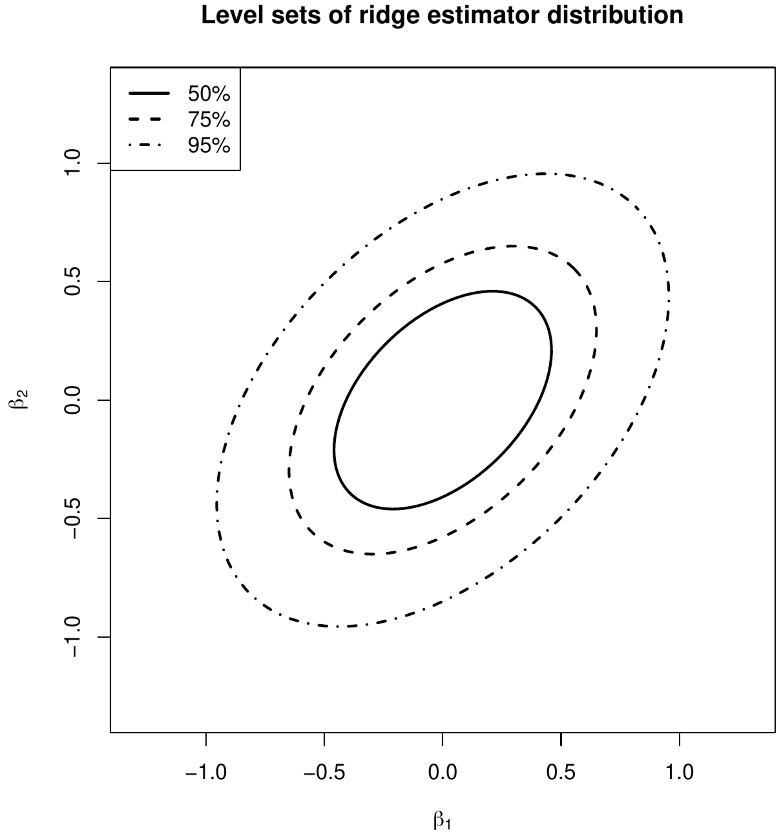
Level sets of the distribution of the ML (left panel) and ridge (right panel) regression estimators.

Example (Variance comparison)

Consider the design matrix:

[[math]] \begin{eqnarray*} \mathbf{X} & = & \left( \begin{array}{rr} -1 & 2 \\ 0 & 1 \\ 2 & -1 \\ 1 & 0 \end{array} \right). \end{eqnarray*} [[/math]]

The variances of the ML and ridge (with [math]\lambda=1[/math]) estimates of the regression coefficients then are:

[[math]] \begin{eqnarray*} \mbox{Var}(\hat{\bbeta}) & = & \sigma^2 \left( \begin{array}{rr} 0.3 & 0.2 \\ 0.2 & 0.3 \end{array} \right) \qquad \mbox{and} \qquad \mbox{Var}[\hat{\bbeta}(\lambda)] \, \, \, = \, \, \, \sigma^2 \left( \begin{array}{rr} 0.1524 & 0.0698 \\ 0.0698 & 0.1524 \end{array} \right). \end{eqnarray*} [[/math]]

These variances can be used to construct levels sets of the distribution of the estimates. The level sets that contain 50%, 75% and 95% of the distribution of the maximum likelihood and ridge regression estimates are plotted in Figure. In line with inequality \ref{form.VarInequalityMLandRidge} the level sets of the ridge regression estimate are smaller than that of the maximum likelihood one. The former thus varies less.

Example (Orthonormal design matrix, continued)

Assume the design matrix [math]\mathbf{X}[/math] is orthonormal. Then, [math]\mbox{Var} ( \hat{\bbeta} ) = \sigma^2 \mathbf{I}_{pp}[/math] and

[[math]] \begin{eqnarray*} \mbox{Var}[ \hat{\bbeta}(\lambda) ] & = & \sigma^2 \mathbf{W}_{\lambda} (\mathbf{X}^{\top} \mathbf{X})^{-1} \mathbf{W}_{\lambda}^{\top} \, \, \, = \, \, \, \sigma^2 (\mathbf{I}_{pp} + \lambda \mathbf{I}_{pp} )^{-1} \mathbf{I}_{pp} [ (\mathbf{I}_{pp} + \lambda \mathbf{I}_{pp} )^{-1} ]^{\top}\, \, \, = \, \, \, \sigma^2 (1 + \lambda )^{-2} \mathbf{I}_{pp}. \end{eqnarray*} [[/math]]

As the penalty parameter [math]\lambda[/math] is non-negative the former exceeds the latter. In particular, the expression after the utmost right equality sign vanishes as [math]\lambda \rightarrow \infty[/math].

The variance of the ridge regression estimator may be decomposed in the same way as its bias (cf. the end of Section Expectation ). There is, however, no contribution of the high-dimensionality of the study design as that is non-random and, consequently, exhibits no variation. Hence, the variance only relates to the variation in the projected subspace [math]\mathcal{R}(\mathbf{X})[/math] as is obvious from:

[[math]] \begin{eqnarray*} \mbox{Var}[ \hat{\bbeta}(\lambda) ] & = & \mbox{Var}[ \mathbf{P}_x \hat{\bbeta}(\lambda) ] \, \, \, = \, \, \, \mathbf{P}_x \mbox{Var}[ \hat{\bbeta}(\lambda) ] \mathbf{P}_x^{\top} \, \, \, = \, \, \, \mbox{Var}[ \hat{\bbeta}(\lambda) ]. \end{eqnarray*} [[/math]]

Perhaps this is seen more clearly when writing the variance of the ridge regression estimator in terms of the matrices that constitute the singular value decomposition of [math]\mathbf{X}[/math]:

[[math]] \begin{eqnarray*} \mbox{Var}[ \hat{\bbeta}(\lambda) ] & = & \mathbf{V}_x (\mathbf{D}_x^{\top} \mathbf{D}_x + \lambda \mathbf{I}_{pp})^{-1} \mathbf{D}_x^{\top} \mathbf{D}_x (\mathbf{D}_x^{\top} \mathbf{D}_x + \lambda \mathbf{I}_{pp})^{-1} \mathbf{V}_x^{\top}. \end{eqnarray*} [[/math]]

High-dimensionally, [math](\mathbf{D}_x^{\top} \mathbf{D}_x)_{jj} = 0[/math] for [math]j=n+1, \ldots, p[/math]. And if [math](\mathbf{D}_x^{\top} \mathbf{D}_x)_{jj} = 0[/math], so is [math][(\mathbf{D}_x^{\top} \mathbf{D}_x + \lambda \mathbf{I}_{pp})^{-1} \mathbf{D}_x^{\top} \mathbf{D}_x \\ (\mathbf{D}_x^{\top} \mathbf{D}_x + \lambda \mathbf{I}_{pp})^{-1}]_{jj} = 0[/math]. Hence, the variance is determined by the first [math]n[/math] columns of [math]\mathbf{V}_x[/math]. When [math]n \lt p[/math], the variance is then to interpreted as the spread of the ridge regression estimator (with the same choice of [math]\lambda[/math]) when the study is repeated with exactly the same design matrix such that the resulting estimator is confined to the same subspace [math]\mathcal{R}(\mathbf{X})[/math]. The following R-script illustrates this by an arbitrary data example (plot not shown):

# set parameters
X      <- matrix(rnorm(2), nrow=1)
betas  <- matrix(c(2, -1), ncol=1)
lambda <- 1

# generate multiple ridge regression estimators with a fixed design matrixs
bHats <- numeric()
for (k in 1:1000){
	Y     <- matrix(X %*% betas + rnorm(1), ncol=1)
	bHats <- rbind(bHats, t(solve(t(X) %*% X + lambda * diag(2)) %*% t(X) %*% Y))
}

# plot the ridge regression estimators
plot(bHats, xlab=expression(paste(hat(beta)[1], "(", lambda, ")", sep="")), 
            ylab=expression(paste(hat(beta)[2], "(", lambda, ")", sep="")), pch=20)

The full distribution of the ridge regression estimator is now known. The estimator, [math]\hat{\bbeta}(\lambda) = (\mathbf{X}^{\top} \mathbf{X} + \lambda \mathbf{I}_{pp})^{-1} \mathbf{X}^{\top} \mathbf{Y}[/math] is a linear estimator, linear in [math]\mathbf{Y}[/math]. As [math]\mathbf{Y}[/math] is normally distributed, so is [math]\hat{\bbeta}(\lambda)[/math]. Moreover, the normal distribution is fully characterized by its first two moments, which are available. Hence:

[[math]] \begin{eqnarray*} \hat{\bbeta}(\lambda) & \sim & \mathcal{N} \{ (\mathbf{X}^{\top} \mathbf{X} + \lambda \mathbf{I}_{pp})^{-1} \mathbf{X}^{\top} \mathbf{X} \, \bbeta, ~\sigma^2 ( \mathbf{X}^{\top} \mathbf{X} + \lambda \mathbf{I}_{pp} )^{-1} \mathbf{X}^{\top} \mathbf{X} [ ( \mathbf{X}^{\top} \mathbf{X} + \lambda \mathbf{I}_{pp} )^{-1} ]^{\top} \}. \end{eqnarray*} [[/math]]

Given [math]\lambda[/math] and [math]\mathbf{X}[/math], the random behavior of the estimator is thus known. In particular, when [math]n \lt p[/math], the variance is semi-positive definite and this [math]p[/math]-variate normal distribution is degenerate, i.e. there is no probability mass outside [math]\mathcal{R}(\mathbf{X})[/math] the subspace of [math]\mathbb{R}^p[/math] spanned by the rows of the [math]\mathbf{X}[/math].

Mean squared error

Previously, we motivated the ridge estimator as an ad hoc solution to collinearity. An alternative motivation comes from studying the Mean Squared Error (MSE) of the ridge regression estimator: for a suitable choice of [math]\lambda[/math] the ridge regression estimator may outperform the ML regression estimator in terms of the MSE. Before we prove this, we first derive the MSE of the ridge estimator and quote some auxiliary results. Note that, as the ridge regression estimator is compared to its ML counterpart, throughout this subsection [math]n \gt p[/math] is assumed to warrant the uniqueness of the latter.

Recall that (in general) for any estimator of a parameter [math]\theta[/math]:

[[math]] \begin{eqnarray*} \mbox{MSE}( \hat{\theta} ) & = & \mathbb{E} [ ( \hat{\theta} - \theta)^2 ] \, \, \, = \, \, \, \mbox{Var}( \hat{ \theta} ) + [\mbox{Bias} ( \hat{\theta} )]^2. \end{eqnarray*} [[/math]]

Hence, the MSE is a measure of the quality of the estimator. The MSE of the ridge regression estimator is:

[[math]] \begin{eqnarray} \mbox{MSE}[\hat{\bbeta}(\lambda)] & = & \mathbb{E} [ (\mathbf{W}_{\lambda} \, \hat{\bbeta} - \bbeta)^{\top} \, (\mathbf{W}_{\lambda} \, \hat{\bbeta} - \bbeta) ] \nonumber \\ & = & \mathbb{E} ( \hat{\bbeta}^{\top} \mathbf{W}_{\lambda}^{\top} \,\mathbf{W}_{\lambda} \, \hat{\bbeta} ) - \mathbb{E} ( \bbeta^{\top} \, \mathbf{W}_{\lambda} \, \hat{\bbeta}) - \mathbb{E} ( \hat{\bbeta}^{\top} \mathbf{W}_{\lambda}^{\top} \, \bbeta) + \mathbb{E} ( \bbeta^{\top} \bbeta) \nonumber \\ & = & \mathbb{E} ( \hat{\bbeta}^{\top} \mathbf{W}_{\lambda}^{\top} \,\mathbf{W}_{\lambda} \, \hat{\bbeta} ) - \mathbb{E} ( \bbeta^{\top} \, \mathbf{W}_{\lambda}^{\top} \mathbf{W}_{\lambda} \, \hat{\bbeta}) - \mathbb{E} ( \hat{\bbeta}^{\top} \mathbf{W}_{\lambda}^{\top} \, \mathbf{W}_{\lambda} \bbeta) + \mathbb{E} ( \bbeta^{\top} \mathbf{W}_{\lambda}^{\top} \,\mathbf{W}_{\lambda} \, \bbeta ) \nonumber \\ & & - \mathbb{E} ( \bbeta^{\top} \mathbf{W}_{\lambda}^{\top} \,\mathbf{W}_{\lambda} \, \bbeta ) + \mathbb{E} ( \bbeta^{\top} \, \mathbf{W}_{\lambda}^{\top} \mathbf{W}_{\lambda} \, \hat{\bbeta}) + \mathbb{E} ( \hat{\bbeta}^{\top} \mathbf{W}_{\lambda}^{\top} \, \mathbf{W}_{\lambda} \bbeta) \nonumber \\ & & - \mathbb{E} ( \bbeta^{\top} \, \mathbf{W}_{\lambda} \, \hat{\bbeta}) - \mathbb{E} ( \hat{\bbeta}^{\top} \mathbf{W}_{\lambda}^{\top} \, \bbeta) + \mathbb{E} ( \bbeta^{\top} \bbeta) \nonumber \\ & = & \mathbb{E} [ ( \hat{\bbeta} - \bbeta )^{\top} \mathbf{W}_{\lambda}^{\top} \, \mathbf{W}_{\lambda} \, (\hat{\bbeta} - \bbeta) ] \nonumber \\ & & - \bbeta^{\top} \mathbf{W}_{\lambda}^{\top} \,\mathbf{W}_{\lambda} \, \bbeta + \bbeta^{\top} \, \mathbf{W}_{\lambda}^{\top} \mathbf{W}_{\lambda} \, \bbeta + \bbeta^{\top} \mathbf{W}_{\lambda}^{\top} \, \mathbf{W}_{\lambda} \bbeta \nonumber \\ & & - \bbeta^{\top} \, \mathbf{W}_{\lambda} \, \bbeta - \bbeta^{\top} \mathbf{W}_{\lambda}^{\top} \, \bbeta + \bbeta^{\top} \bbeta \nonumber \\ & = & \mathbb{E} [ ( \hat{\bbeta} - \bbeta )^{\top} \mathbf{W}_{\lambda}^{\top} \, \mathbf{W}_{\lambda} \, (\hat{\bbeta} - \bbeta) ] + \bbeta^{\top} (\mathbf{W}_{\lambda} - \mathbf{I}_{pp})^{\top} (\mathbf{W}_{\lambda} - \mathbf{I}_{pp}) \bbeta \nonumber \\ & = & \sigma^2 \, \mbox{tr} [ \mathbf{W}_{\lambda} \, (\mathbf{X}^{\top} \mathbf{X})^{-1} \, \mathbf{W}_{\lambda}^{\top} ] + \bbeta^{\top} (\mathbf{W}_{\lambda} - \mathbf{I}_{pp})^{\top} (\mathbf{W}_{\lambda} - \mathbf{I}_{pp}) \bbeta. \label{form.ridgeMSE} \end{eqnarray} [[/math]]

In the last step we have used [math]\hat{\bbeta} \sim \mathcal{N}[ \bbeta, \sigma^2 \, (\mathbf{X}^{\top} \mathbf{X})^{-1} ][/math] and the expectation of the quadratic form of a multivariate random variable [math]\vvarepsilon \sim \mathcal{N}(\mmu_{\varepsilon}, \SSigma_{\varepsilon})[/math] that for a nonrandom symmetric positive definite matrix [math]\LLambda[/math] is (cf. ):

[[math]] \begin{eqnarray*} \mathbb{E} ( \vvarepsilon^{\top} \LLambda \, \vvarepsilon) & = & \mbox{tr} ( \LLambda \SSigma_{\varepsilon}) + \mmu_{\varepsilon}^{\top} \LLambda \mmu_{\varepsilon}, \end{eqnarray*} [[/math]]

of course replacing [math]\vvarepsilon[/math] by [math]\hat{\bbeta}[/math] in this expectation. The first summand in the final derived expression for [math]\mbox{MSE}[\hat{\bbeta}(\lambda)][/math] is the sum of the variances of the ridge estimator, while the second summand can be thought of the “squared bias” of the ridge estimator. In particular, [math]\lim_{\lambda \rightarrow \infty} \mbox{MSE}[\hat{\bbeta}(\lambda)] = \bbeta^{\top} \bbeta[/math], which is the squared biased for an estimator that equals zero (as does the ridge regression estimator in the limit).

Example Orthonormal design matrix

Assume the design matrix [math]\mathbf{X}[/math] is orthonormal. Then, [math]\mbox{MSE}[ \hat{\bbeta} ] = p \, \sigma^2[/math] and

[[math]] \begin{eqnarray*} \mbox{MSE}[ \hat{\bbeta}(\lambda) ] & = & p \, \sigma^2 (1+ \lambda)^{-2} + \lambda^2 (1+ \lambda)^{-2} \bbeta^{\top} \bbeta. \end{eqnarray*} [[/math]]

The latter achieves its minimum at: [math]\lambda = p \sigma^2 / \bbeta^{\top} \bbeta[/math].

The following theorem and proposition are required for the proof of the main result.

Theorem 1 of

Let [math]\hat{\ttheta}_1[/math] and [math]\hat{\ttheta}_2[/math] be (different) estimators of [math]\ttheta[/math] with second order moments:

[[math]] \begin{eqnarray*} \mathbf{M}_k & = & \mathbb{E} [ (\hat{\ttheta}_k - \ttheta) (\hat{\ttheta}_k - \ttheta)^{\top} ] \qquad \mbox{for } k=1,2, \end{eqnarray*} [[/math]]

and

[[math]] \begin{eqnarray*} \mbox{MSE}(\hat{\ttheta}_k) & = & \mathbb{E} [ (\hat{\ttheta}_k - \ttheta)^{\top} \mathbf{A} (\hat{\ttheta}_k - \ttheta) ] \qquad \mbox{for } k=1,2, \end{eqnarray*} [[/math]]

where [math]\mathbf{A} \succeq 0[/math]. Then, [math]\mathbf{M}_1 - \mathbf{M}_2 \succeq 0[/math] if and only if [math]\mbox{MSE}(\hat{\ttheta}_1) - \mbox{MSE}(\hat{\ttheta}_2) \geq 0[/math] for all [math]\mathbf{A} \succeq 0[/math].

Proposition

Let [math]\mathbf{A}[/math] be a [math]p \times p[/math]-dimensional, positive definite matrix, [math]\mathbf{b}[/math] be a nonzero [math]p[/math] dimensional vector, and [math]c \in \mathbb{R}_+[/math]. Then, [math]c \mathbf{A} - \mathbf{b} \mathbf{b}^{\top} \succ 0[/math] if and only if [math]\mathbf{b}^{\top} \mathbf{A}^{-1} \mathbf{b} \lt c[/math].

We are now ready to proof the main result, formalized as Theorem, that for some [math]\lambda[/math] the ridge regression estimator yields a lower MSE than the ML regression estimator. Question provides a simpler (?) but more limited proof of this result.

Theorem 2 of

There exists [math]\lambda \gt 0[/math] such that [math]\mbox{MSE}[\hat{\bbeta}(\lambda)] \lt \mbox{MSE}[\hat{\bbeta}(0)] = \mbox{MSE}(\hat{\bbeta})[/math].

Show Proof

The second order moment matrix of the ridge estimator is:

[[math]] \begin{eqnarray*} \mathbf{M} (\lambda) & := & \mathbb{E} [ (\hat{\bbeta}(\lambda) - \bbeta) (\hat{\bbeta} (\lambda) - \bbeta)^{\top} ] \\ & = & \mathbb{E} \{ \hat{\bbeta}(\lambda) [\hat{\bbeta}(\lambda)]^{\top} \} - \mathbb{E} [ \hat{\bbeta}(\lambda) ] \{ \mathbb{E} [ \hat{\bbeta}(\lambda) ] \}^{\top} + \mathbb{E} [\hat{\bbeta} (\lambda) - \bbeta)] \{ \mathbb{E} [\hat{\bbeta} (\lambda) - \bbeta)] \}^{\top} \\ & = & \mbox{Var}[ \hat{\bbeta}(\lambda) ] + \mathbb{E} [\hat{\bbeta} (\lambda) - \bbeta)] \{ \mathbb{E} [\hat{\bbeta} (\lambda) - \bbeta)] \}^{\top}. \end{eqnarray*} [[/math]]

Then:

[[math]] \begin{eqnarray*} \mathbf{M} ( 0 ) - \mathbf{M}(\lambda) & = & \sigma^2 (\mathbf{X}^{\top} \mathbf{X})^{-1} - \sigma^2 \mathbf{W}_{\lambda} (\mathbf{X}^{\top} \mathbf{X})^{-1} \mathbf{W}_{\lambda}^{\top} - (\mathbf{W}_{\lambda} - \mathbf{I}_{pp}) \bbeta \bbeta^{\top} (\mathbf{W}_{\lambda} -\mathbf{I}_{pp})^{\top} \\ & = & \sigma^2 \mathbf{W}_{\lambda} (\mathbf{X}^{\top} \mathbf{X})^{-1} (\mathbf{X}^{\top} \mathbf{X}+ \lambda \mathbf{I}_{pp}) (\mathbf{X}^{\top} \mathbf{X})^{-1} (\mathbf{X}^{\top} \mathbf{X}+ \lambda \mathbf{I}_{pp}) (\mathbf{X}^{\top} \mathbf{X})^{-1} \mathbf{W}_{\lambda}^{\top} \\ & & - \sigma^2 \mathbf{W}_{\lambda} (\mathbf{X}^{\top} \mathbf{X})^{-1} \mathbf{W}_{\lambda}^{\top} - (\mathbf{W}_{\lambda} - \mathbf{I}_{pp}) \bbeta \bbeta^{\top} (\mathbf{W}_{\lambda} -\mathbf{I}_{pp})^{\top} \\ & = & \sigma^2 \mathbf{W}_{\lambda} [ 2 \, \lambda \, (\mathbf{X}^{\top} \mathbf{X})^{-2} + \lambda^2 (\mathbf{X}^{\top} \mathbf{X})^{-3} ] \mathbf{W}_{\lambda}^{\top} \\ & & - \lambda^2 (\mathbf{X}^{\top} \mathbf{X} + \lambda \mathbf{I}_{pp})^{-1} \bbeta \bbeta^{\top} [ (\mathbf{X}^{\top} \mathbf{X} + \lambda \mathbf{I}_{pp})^{-1} ]^{\top} \\ & = & \sigma^2 ( \mathbf{X}^{\top} \mathbf{X} + \lambda \mathbf{I}_{pp} )^{-1} [ 2 \, \lambda \, \mathbf{I}_{pp} + \lambda^2 (\mathbf{X}^{\top} \mathbf{X})^{-1} ] [ (\mathbf{X}^{\top} \mathbf{X} + \lambda \mathbf{I}_{pp})^{-1} ]^{\top} \\ & & - \lambda^2 ( \mathbf{X}^{\top} \mathbf{X} + \lambda \mathbf{I}_{pp} )^{-1} \bbeta \bbeta^{\top} [ ( \mathbf{X}^{\top} \mathbf{X} + \lambda \mathbf{I}_{pp})^{-1} ]^{\top} \\ & = & \lambda ( \mathbf{X}^{\top} \mathbf{X} + \lambda \mathbf{I}_{pp})^{-1} [ 2 \, \sigma^2 \, \mathbf{I}_{pp} + \lambda \sigma^2 (\mathbf{X}^{\top} \mathbf{X})^{-1} - \lambda \bbeta \bbeta^{\top} ] [ (\mathbf{X}^{\top} \mathbf{X} + \lambda \mathbf{I}_{pp} )^{-1} ]^{\top}. \end{eqnarray*} [[/math]]

This is positive definite if and only if [math] 2 \, \sigma^2 \, \mathbf{I}_{pp} + \lambda \sigma^2 (\mathbf{X}^{\top} \mathbf{X})^{-1} - \lambda \bbeta \bbeta^{\top} \succ 0[/math]. Hereto it suffices to show that [math]2 \, \sigma^2 \, \mathbf{I}_{pp} - \lambda \bbeta \bbeta^{\top} \succ 0[/math]. By Proposition this holds for [math]\lambda[/math] such that [math]2 \sigma^2 (\bbeta^{\top} \bbeta)^{-1} \gt \lambda[/math]. For these [math]\lambda[/math], we thus have [math]\mathbf{M} ( 0 ) - \mathbf{M}(\lambda)[/math]. Application of Theorem now concludes the proof. ■

This result of is generalized by to the class of design matrices [math]\mathbf{X}[/math] with [math]\mbox{rank}(\mathbf{X}) \lt p[/math].

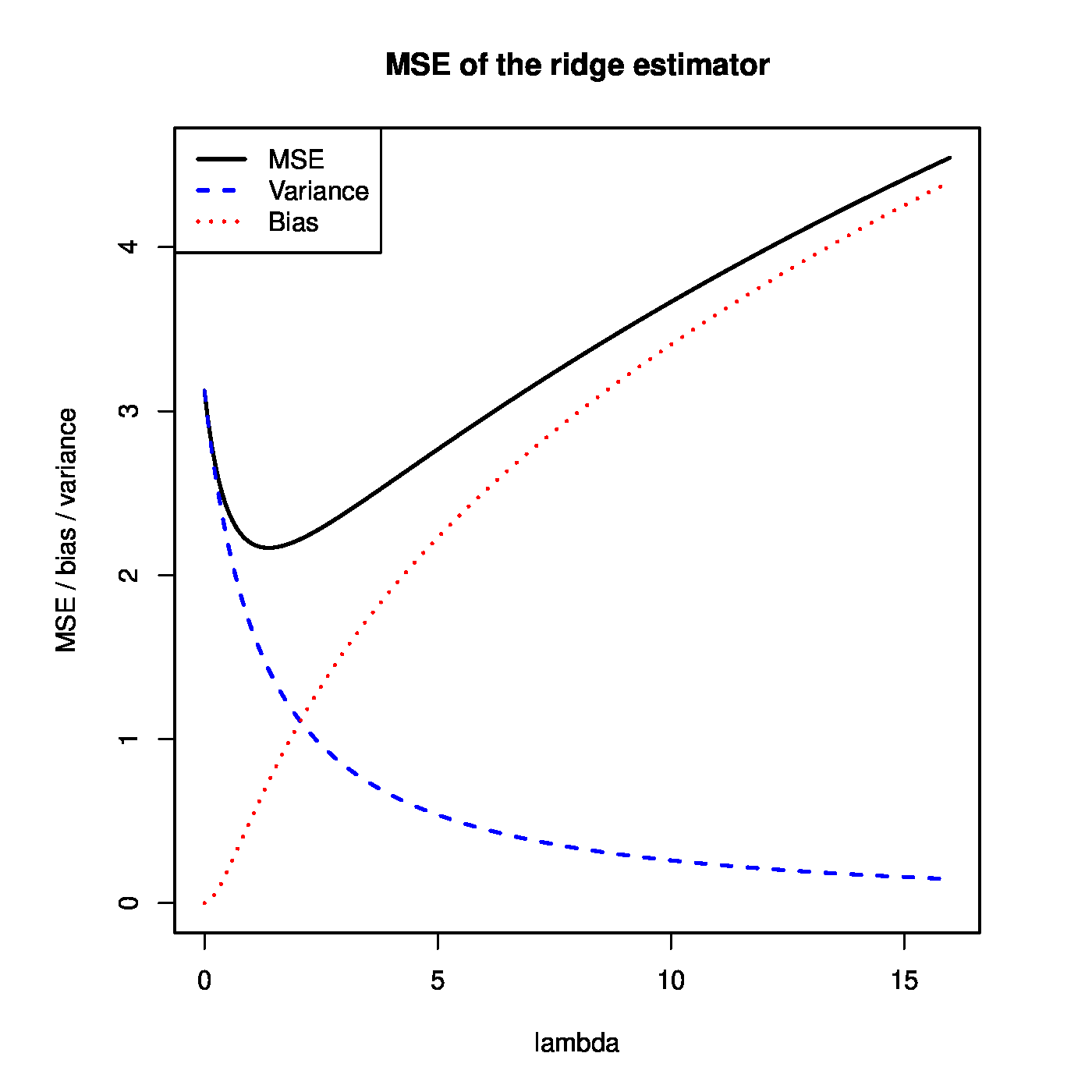
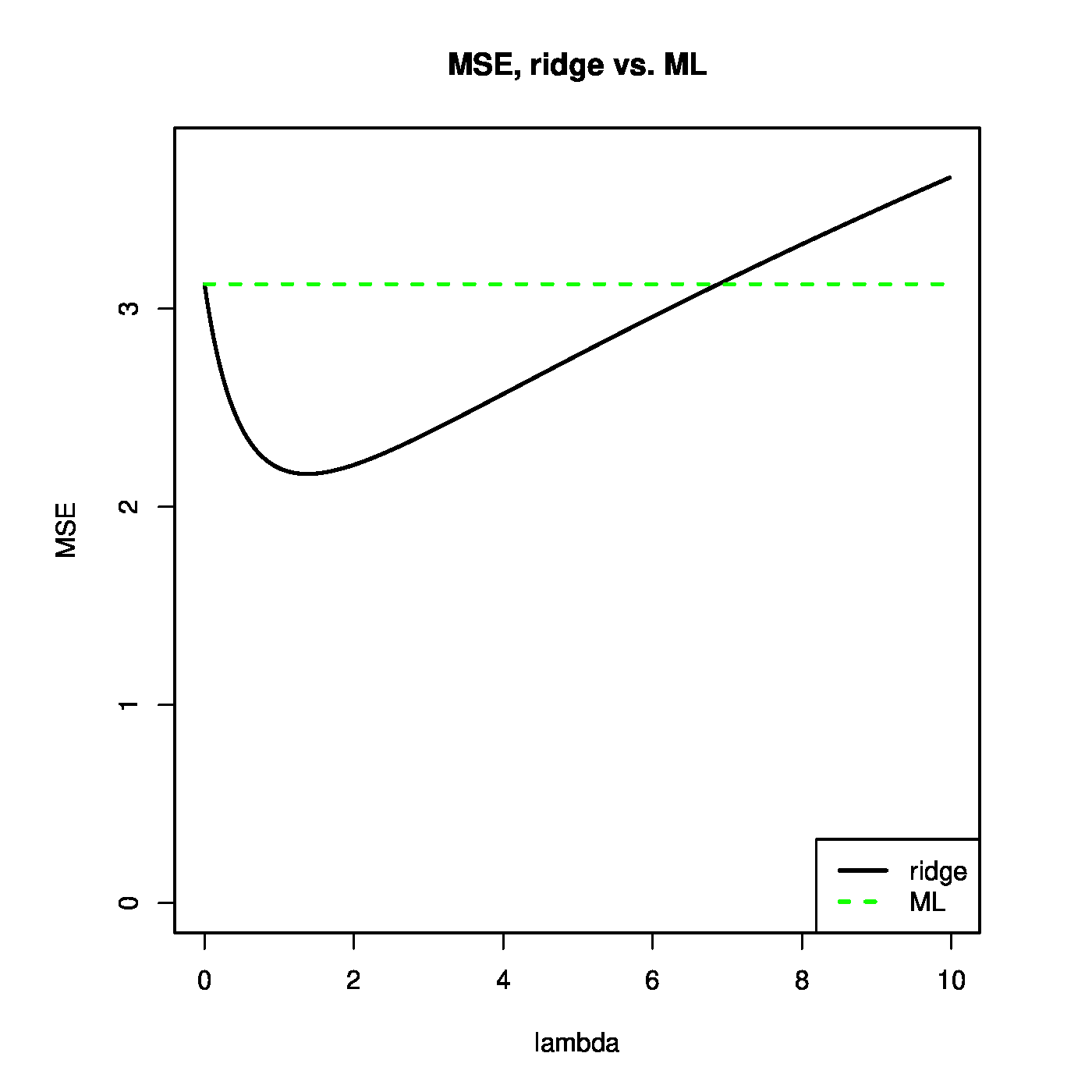
Theorem can be used to illustrate that the ridge regression estimator strikes a balance between the bias and variance. This is illustrated in the left panel of Figure. For small [math]\lambda[/math], the variance of the ridge estimator dominates the MSE. This may be understood when realizing that in this domain of [math]\lambda[/math] the ridge estimator is close to the unbiased ML regression estimator. For large [math]\lambda[/math], the variance vanishes and the bias dominates the MSE. For small enough values of [math]\lambda[/math], the decrease in variance of the ridge regression estimator exceeds the increase in its bias. As the MSE is the sum of these two, the MSE first decreases as [math]\lambda[/math] moves away from zero. In particular, as [math]\lambda = 0[/math] corresponds to the ML regression estimator, the ridge regression estimator yields a lower MSE for these values of [math]\lambda[/math]. In the right panel of Figure [math]\mbox{MSE}[ \hat{\bbeta}(\lambda)] \lt \mbox{MSE}[ \hat{\bbeta}(0)][/math] for [math]\lambda \lt 7[/math] (roughly) and the ridge estimator outperforms the ML estimator.

Left panel: mean squared error, and its ‘bias’ and ‘variance’ parts, of the ridge regression estimator (for artificial data). Right panel: mean squared error of the ridge and ML estimator of the regression coefficient vector (for the same artificial data).

Besides another motivation behind the ridge regression estimator, the use of Theorem is limited. The optimal choice of [math]\lambda[/math] depends on the quantities [math]\bbeta[/math] and [math]\sigma^2[/math]. These are unknown in practice. Then, the penalty parameter is chosen in a data-driven fashion (see e.g. Section Cross-validation and various other places).

Theorem may be of limited practical use, it does give insight in when the ridge regression estimator may be preferred over its ML counterpart. Ideally, the range of penalty parameters for which the ridge regression estimator outperforms -- in the MSE sense -- the ML regression estimator is as large as possible. The factors that influence the size of this range may be deduced from the optimal penalty [math]\lambda_{\mbox{{\tiny opt}}} = \sigma^2 (\bbeta^{\top} \bbeta / p)^{-1}[/math] found under the assumption of an orthonormal [math]\mathbf{X}[/math] (see Example). But also from the bound on the penalty parameter, [math]\lambda_{\mbox{{\tiny max}}} = 2 \sigma^2 (\bbeta^{\top} \bbeta )^{-1}[/math] such that [math]MSE[\hat{\bbeta}(\lambda)] \lt MSE[\hat{\bbeta}(0)][/math] for all [math]\lambda \in (0, \lambda_{\mbox{{\tiny max}}})[/math], derived in the proof of Theorem. Firstly, an increase of the error variance [math]\sigma^2[/math] yields a larger [math]\lambda_{\mbox{{\tiny opt}}}[/math] and [math]\lambda_{\mbox{{\tiny max}}}[/math]. Put differently, more noisy data benefits the ridge regression estimator. Secondly, [math]\lambda_{\mbox{{\tiny opt}}}[/math] and [math]\lambda_{\mbox{{\tiny max}}}[/math] also become larger when their denominators decreases. The denominator [math]\bbeta^{\top} \bbeta / p[/math] may be viewed as an estimator of the ‘signal’ variance ‘[math]\sigma^2_{\beta}[/math]’. A quick conclusion would be that ridge regression profits from less signal. But more can be learned from the denominator. Contrast the two regression parameters [math]\bbeta_{\mbox{{\tiny unif}}} = \mathbf{1}_p[/math] and [math]\bbeta_{\mbox{{\tiny sparse}}}[/math] which comprises of only zeros except the first element which equals [math]p[/math], i.e. [math]\bbeta_{\mbox{{\tiny sparse}}} = (p, 0, \ldots, 0)^{\top}[/math]. Then, the [math]\bbeta_{\mbox{{\tiny unif}}}[/math] and [math]\bbeta_{\mbox{{\tiny sparse}}}[/math] have comparable signal in the sense that [math]\sum_{j=1}^p \beta_j = p[/math]. The denominator of [math]\lambda_{\mbox{{\tiny opt}}}[/math] corresponding both parameters equals [math]1[/math] and [math]p[/math], respectively. This suggests that ridge regression will perform better in the former case where the regression parameter is not dominated by a few elements but rather all contribute comparably to the explanation of the variation in the response. Of course, more factors contribute. For instance, collinearity among the columns of [math]\mathbf{X}[/math], which gave rise to ridge regression in the first place.

Theorem can also be used to conclude on the biasedness of the ridge regression estimator. The Gauss-Markov theorem states (under some assumptions) that the ML regression estimator is the best linear unbiased estimator (BLUE) with the smallest MSE. As the ridge regression estimator is a linear estimator and outperforms (in terms of MSE) this ML estimator, it must be biased (for it would otherwise refute the Gauss-Markov theorem).

General References

van Wieringen, Wessel N. (2021). "Lecture notes on ridge regression". arXiv:1509.09169 [stat.ME].

References

- Shao, J. and Deng, X. (2012).Estimation in high-dimensional linear models with deterministic design matrices.The Annals of Statistics, 40(2), 812--831
- Mathai, A. M. and Provost, S. B. (1992).Quadratic Forms in Random Variables: Theory and Applications.Dekker
- 3.0 3.1 3.2 Theobald, C. M. (1974).Generalizations of mean square error applied to ridge regression.Journal of the Royal Statistical Society. Series B (Methodological), 36(1), 103--106
- 4.0 4.1 Farebrother, R. W. (1976).Further results on the mean square error of ridge regression.Journal of the Royal Statistical Society, Series B (Methodological), pages 248--250
- Rao, C. R. (1973).Linear Statistical Inference and its Applications.John Wiley & Sons