The Black-Scholes Theory

\label{chapt:blackScholes} This section builds a pricing theory around the assumptions of no-arbitrage with perfect liquidity and trades occurring in continuous time. The Black-Scholes model is a complete market, and there turns out to be a fairly general class of partial differential equations (PDEs) that can price many contingent claims. The focus of Black-Scholes theory is often on European call and put options, but exotics such as the Asian and the exchange option are simple extensions of the basic formulae. The issues with American options are covered later in Section American Options and Optimality of Early Exercise.

The Black-Scholes Model

The Black-Scholes model assumes a market consisting of a single risky asset and a risk-free bank account. This market is given by the equations

[[math]] \begin{eqnarray*} \frac{dS_t}{S_t}&=&\mu dt+\sigma dW_t\qquad\hbox{geometric Brownian-Motion}\\ dB_t&=&rB_tdt\qquad\qquad\hbox{non-stochastic} \end{eqnarray*} [[/math]]

where [math]W_t[/math] is Brownian motion as described in Chapter and the interpretation of the parameters is as follows:

[[math]] \begin{align*} &\mu\hbox{ is the expected rate of return in the risk asset,}\\ &\sigma \gt 0\hbox{ is the volatility of the risky asset,}\\ &r\geq0\hbox{ is the bank's rate of interest.} \end{align*} [[/math]]

It turns out that this market is particularly well-suited for pricing options and other variations, as well as analyzing basic risks associated with the writing of such contracts. Even though this market is an oversimplification of real life, it is still remarkable how a such a parsimonious model is able to capture so much of the very essence of the risky behavior in the markets. In particular, the parameter [math]\sigma[/math] will turn out to be a hugely important factor in secondary markets for options, swaps, etc. The default focus in these notes will be the European call option with strike [math]K[/math] and maturity [math]T[/math], that is, a security that pays

[[math]](S_T-K)^+\doteq\max(S_T-K,0)\ ,[[/math]]

with strike and contract price agreed upon at some earlier time [math]t \lt T[/math]. In general, the price of any European derivative security with payoff [math]\psi(S_T)[/math] (i.e. a derivative with payoff determined by the terminal value of risky asset) will be a function of the current time and the current asset price,

[[math]]C(t,S_t) = \hbox{ price of derivative security.}[[/math]]

The fact that the price can be written a function of [math]t[/math] and [math]S_t[/math] irrespective of [math]S[/math]'s history is due to the fact the model is Markov. Through an arbitrage argument we will arrive at a PDE for the pricing function [math]C[/math]. Pricing equations for general non-European derivatives (such as the Asian option discussed in Section Asian Options) are determined on a case-by-case basis.

Self-Financing Portfolio

Let [math]V_t[/math] denote the \$-value of a portfolio with shares in the risk asset and the rest of it's value in the risk-free bank account. At any time the portfolio can be written as

[[math]]V_t=\alpha_tS_t+\beta_t[[/math]]

where [math]\alpha_t[/math] is the number of shares in [math]S_t[/math] (could be any real number) and [math]\beta_t[/math] is the \$-amount in bank. The key characteristic that will be associated with [math]V[/math] throughout these notes is the following condition:

Definition

The portfolio [math]V_t[/math] is self-financing if

[[math]]dV_t = \alpha_tdS_t+r\beta_tdt[[/math]]

with [math]\beta_t = V_t-\alpha_tS_t[/math].

The self-financing condition is not entirely obvious at first, but it helps to think of one's personal decision-making in a financial market. Usually, one chooses a portfolio allocation in stocks and bonds, and then allows a certain amount of change to occur in the market before adjusting their allocation. If you don't remove any cash for consumption and you don't inject any cash for added investment, then your portfolio is self-financing. Indeed, in discrete time the self-financing condition is

[[math]]V_{t_{n+1}} = V_{t_n}+\alpha_{t_n}(S_{t_{n+1}}-S_{t_n})+(e^{r\Delta t}-1)\beta_{t_n}[[/math]]

where [math]\Delta t = t_{n+1}-t_n[/math]. This becomes the condition described in Definition as [math]\Delta t\searrow 0[/math].

The Black-Scholes Equation

For general functions [math]f(t,s)[/math], the It\^o lemma for the geometric Brownian motion process is

[[math]]df(t,S_t) = \left(\frac{\partial}{\partial t}+\mu S_t\frac{\partial}{\partial s}+\frac{\sigma^2S_t^2}{2}\frac{\partial^2}{\partial s^2}\right)f(t,S_t)dt+\sigma S_t\frac{\partial}{\partial s}f(t,S_t)dW_t[[/math]]

(recall equation eq:itoLemma from Chapter). Hence, applying the It\^o lemma to the price function [math]C(t,S_t)[/math], the dynamics of the option and the self-financing portfolio are

[[math]] \begin{eqnarray} \label{eq:dC} dC(t,S_t)&=&\left(\frac{\partial}{\partial t}+\mu S_t\frac{\partial}{\partial s}+\frac{\sigma^2S_t^2}{2}\frac{\partial^2}{\partial s^2}\right)C(t,S_t)dt+\sigma S_t\frac{\partial}{\partial s}C(t,S_t)dW_t\\ \nonumber &&\\ \label{eq:dV} dV_t &=&\alpha_tdS_t+r\beta_tdt\ . \end{eqnarray} [[/math]]

The idea is to find [math]\alpha_t[/math] that can be known to us at time [math]t[/math] (given our observed history of prices) so that [math]V_t[/math] replicates [math]C(t,S_t)[/math] as closely as possible. Setting [math]\alpha_t=\frac{\partial}{\partial s}C(t,S_t)[/math] and [math]\beta_t = V_t-\alpha_tS_t[/math], then buying the portfolio and shorting [math]C[/math] gets a risk-less portfolio

[[math]]d(V_t-C(t,S_t)) = r\left(V_t-S_t\frac{\partial}{\partial s}C(t,S_t)\right)dt-\left(\frac{\partial}{\partial t}+\frac{\sigma^2S_t^2}{2}\frac{\partial^2}{\partial s^2}\right)C(t,S_t)dt[[/math]]

and by arbitrage arguments, this must be equal to the risk-free rate,

[[math]]=r(V_t-C(t,S_t))dt\ .[[/math]]

Hence, we arrive at the Black-Scholes PDE

[[math]] \begin{equation} \label{eq:BSpde} \left(\frac{\partial}{\partial t}+\frac{\sigma^2s^2}{2}\frac{\partial^2}{\partial s^2}+rs\frac{\partial}{\partial s}-r\right)C(t,s) = 0 \end{equation} [[/math]]

with [math]C(T,s) = \psi(s)[/math] (recall we denote payoff function for general European claim with function [math]\psi(s)[/math]). The power of the Black -Scholes PDE is that it replicates perfectly. Observe: if [math]V_0 = C(0,S_0)[/math], then

[[math]]d(V_t-C(t,S_t)) = 0\qquad\forall t\leq T,[[/math]]

and so [math]V_T = C(T,S_T) =\psi(S_T)[/math]. In fact, it can be shown that any contingent claim (not just Europeans) is replicable under the Black-Scholes model. Hence, the market is complete.

Feynman-Kac, the EMM, & Heat Equations

Feynman-Kac is a probabilistic formula for solving PDEs like \eqref{eq:BSpde}. It also has financial meaning because it explicitly provides a unique equivalent martingale measure (EMM). Since we have assume no-arbitrage, the 1st Fundamental theorem of asset pricing (see Section) necessarily asserts the existence of an EMM. The structure of this probability measure is given to us by the Feynman-Kac formula:

Proposition (Feynman-Kac)

The solution to the Black-Scholes PDE of \eqref{eq:BSpde} is the expectation

[[math]]C(t,s) = e^{-r(T-t)}\mathbb E^Q[\psi(S_T)|S_t=s][[/math]]

where [math]\mathbb E^Q[/math] is an EMM under which [math]e^{r(T-t)}S_t[/math] is a martingale,

[[math]]dS_t = rS_tdt+\sigma S_tdW_t^Q\ ,[[/math]]

with [math]W_t^Q \doteq \frac{\mu-r}{\sigma}t+W_t[/math] being Brownian motion under the EMM.

Non-Smooth Payoffs. For call options, the function [math]\psi[/math] is not twice differentiable nor does it have compact support, so Proposition is not a direct application of Feynman-Kac as stated in Proposition of Chapter. There needs to be a further massaging of PDE to show that the formula holds for this special case. It is quite technical, but the end result is that Feynman-Kac applies to most payoffs of financial assets for log-normal models.\\

Uniqueness. The uniqueness of the EMM in Proposition can be argued by using the uniqueness of solutions to \eqref{eq:BSpde}. The conclusion that the EMM is unique and that the market is complete.

Relationship with Heat Equation. The Black-Scholes PDE \eqref{eq:BSpde} is a type of heat equation from physics. The basic heat equation is

[[math]]\frac{\partial}{\partial t}u(t,x) = \sigma^2\frac{\partial^2}{\partial x^2}u(t,x)[[/math]]

with some initial condition [math]u|_{t=0} = f[/math]. Solutions to the heat equation are interpreted as the evolution of Brownian motion's probability distribution. In the same manner that passage of time will coincide with the diffusion of heat from a source, the heat equation can describe the diffusion of possible trajectories of Brownian motion away from their common starting point of [math]W_0 = 0[/math]. Equation \eqref{eq:BSpde} obviously has some extra term and an ‘[math]s[/math]’ in front of the 2nd derivative, but a change of variables of [math]\tau=T-t[/math] and [math]x=\log(s)[/math] leads to a representation of the solution as

[[math]]\widetilde C(\tau,x) = C(T-\tau,e^x)[[/math]]

where [math]C[/math] solves the Black-Scholes PDE. Doing the calculus we arrive at a more basic PDE for [math]\widetilde C[/math],

[[math]]\frac{\partial}{\partial\tau}\widetilde C(\tau,x) = \frac{\sigma^2}{2}\frac{\partial^2}{\partial x^2}\widetilde C(\tau,x)+\left(b\frac{\partial}{\partial x}-r\right)\widetilde C(\tau,x)[[/math]]

with initial condition [math]C(0,x) = \psi(e^x)[/math], and with [math]b=\frac{2r-\sigma^2}{2}[/math]. Hence Black-Scholes is a heat equation with drift [math]b\frac{\partial}{\partial x}\widetilde C(\tau,x)[/math], and decay [math]r\widetilde C(\tau,x)[/math].

The Black-Scholes Call Option Formula

Let [math]\psi(s) = (s-K)^+[/math]. From Feynman-Kac we have

[[math]]C(t,s) = e^{-r(T-t)}\mathbb E^Q[(S_T-K)^+|S_t=s][[/math]]

with [math]dS_t = rS_tdt+\sigma S_tdW_t^Q[/math]. Through a verification with It\^o's Lemma we can see that underlying's value at time of maturity can be written as a log-normal random variable,

[[math]]S_T = S_t\exp\left(\left(r-\frac 12\sigma^2\right)(T-t)+\sigma (W_T-W_t)\right)\ .[[/math]]

And so [math]\log(S_T/S_t)[/math] is in fact normally distributed under the risk-neutral measure,

[[math]]\log(S_T/S_t)\sim\mathcal N\left( \left(r-\frac 12\sigma^2\right)(T-t),\sigma^2(T-t)\right)\ .[[/math]]

Hence, we compute the expectation for [math]\psi(s) = (s-K)^+[/math],

[[math]]\mathbb E^Q\{(S_T-K)^+|S_t=s\}[[/math]]

[[math]] =\underbrace{ \frac{S_t}{\sqrt{2\pi\sigma^2(T-t)}}\int_{\log(K/S_t)}^\infty e^xe^{-\frac12\left(x- \left(r-\frac 12\sigma^2\right)(T-t)\right)^2/(\sigma^2(T-t))}dx}_{=(\dagger)}[[/math]]

[[math]]-\underbrace{K\mathbb Q(\log(S_T/S_t) \gt \log(K/S_t))}_{=(\star)} [[/math]]

where [math]\mathbb Q[/math] is the risk-neutral probability measure.

[math]\mathbf{(\dagger).}[/math] First compute [math](\dagger)[/math] (W.L.O.G. for [math]t=0[/math]):

[[math]](\dagger) = \frac{S_0}{\sqrt{2\pi\sigma^2 T}}\int_{\log(K/S_0)}^\infty e^x e^{-\frac 12\left(\frac{x-(r-\frac 12\sigma^2)T}{\sigma\sqrt T}\right)^2}dx[[/math]]

[[math]]= \frac{S_0}{\sqrt{2\pi\sigma^2 T}}\int_{\log(K/S_0)}^\infty e^{-\frac{1}{2\sigma^2T}\left(-2x^2\sigma^2T+x^2-2x(r-.5\sigma^2)T+((r-.5\sigma^2)T)^2\right)}dx[[/math]]

[[math]]= \frac{S_0}{\sqrt{2\pi\sigma^2 T}}\int_{\log(K/S_0)}^\infty e^{-\frac{1}{2\sigma^2T}\left(x^2-2x(r+.5\sigma^2)T+((r-.5\sigma^2)T)^2\right)}dx[[/math]]

[[math]]= \frac{S_0e^{rT}}{\sqrt{2\pi\sigma^2 T}}\int_{\log(K/S_0)}^\infty e^{-\frac{1}{2\sigma^2T}\left(x^2-(r+.5\sigma^2)T\right)^2}dx[[/math]]

change of variables [math]v = \frac{x-(r+.5\sigma^2)T}{\sigma\sqrt T}[/math], [math]dv = dx/(\sigma\sqrt T)[/math], so that

[[math]](\dagger) = \frac{S_0e^{rT}}{\sqrt{2\pi}}\int_{(\log(K/S_0)-(r+.5\sigma^2)T)/(\sigma\sqrt T)}^\infty e^{\frac 12 v^2}dv[[/math]]

[[math]]= S_0e^{rT}\left(1 - \frac{1}{\sqrt{2\pi}}\int_{-\infty}^{(\log(K/S_0)-(r+.5\sigma^2)T)/(\sigma\sqrt T)} e^{\frac 12 v^2}dv\right)[[/math]]

[[math]]=S_0e^{rT}\left(1 - N(-d_1)\right)[[/math]]

where [math]d_1 = \frac{\log(S_0/K)+(r+.5\sigma^2)T}{\sigma\sqrt T}[/math] and [math]N(\cdot)[/math] is the standard normal CDF. But the normal CDF has the property that [math]N(-x) = 1-N(x)[/math], so

[[math]](\dagger) = S_0e^{rT}N(d_1)\ .[[/math]]

[math]\mathbf{(\star)}.[/math] Then, computing [math](\star)[/math] is much simpler,

[[math]](\star) = K\mathbb Q\left(\log(S_T/S_0)\geq \log(K/S_0)\right)[[/math]]

[[math]]=K\mathbb Q\left(\frac{\log(S_T/S_0)-(r-.5\sigma^2)T}{\sigma\sqrt T}\geq\frac{ \log(K/S_0)-(r-.5\sigma^2)T}{\sigma\sqrt T}\right)[[/math]]

[[math]]=K\left(1 - \mathbb Q\left(\frac{\log(S_T/S_0)-(r-.5\sigma^2)T}{\sigma\sqrt T}\leq\frac{ \log(K/S_0)-(r-.5\sigma^2)T}{\sigma\sqrt T}\right)\right)[[/math]]

[[math]]=K\left(1-N(-d_2) \right)= KN(d_2)[[/math]]

where [math]d_2 =\frac{ \log(S_0/K)+(r-.5\sigma^2)T}{\sigma\sqrt T}=d_1-\sigma\sqrt T[/math]. Hence, we have the Black-Scholes formula for a European Call Option,

Proposition (Black-Scholes Call Option Formula)

The call option on [math]S_T[/math] with strike [math]K[/math] at time [math]t[/math] with price [math]S_t[/math] is given by

[[math]]C(t,S_t) = S_tN(d_1)-Ke^{-r(T-t)}N(d_2)[[/math]]

where [math]N(\cdot)[/math] is the standard normal CDF and

[[math]] \begin{align*} &d_1 = \frac{\log(S_t/K)+(r+.5\sigma^2)(T-t)}{\sigma\sqrt{T-t}} \\ &d_2 = d_1-\sigma\sqrt{T-t}\ . \end{align*} [[/math]]

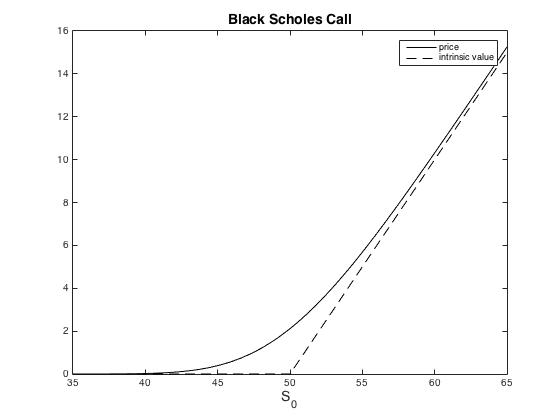
A plot of the Black-Scholes call option price with [math]K=50[/math], [math]r=.02[/math], [math]T=3/12[/math], and [math]\sigma=.2[/math] with varying [math]S_0[/math] is shown in Figure.

The Black-Scholes call price with [math]K=50[/math], [math]r=.02[/math], [math]T=3/12[/math], and [math]\sigma=.2[/math]. Intrinsic value refers to the payoff if exercised now, [math](S_0-K)^+[/math].

Put-Call Parity and the Put Option Formula

It is straight forward to verify the relationship

[[math]] \begin{equation} \label{eq:PCterminal} (S_T-K)^+-(K-S_T)^+ = S_T-K\ . \end{equation} [[/math]]

Then applying the risk-neutral expectionan [math]e^{-r(T-t)}\mathbb E_t^Q[/math] to both sides of \eqref{eq:PCterminal} to get the put-call parity,

[[math]] \begin{equation} \label{eq:PCparity} C(t,S_t)-P(t,S_t) = S_t-Ke^{-r(T-t)} \end{equation} [[/math]]

where [math]C(t,S_t)[/math] is the price of a European call option and [math]P(t,S_t)[/math] the price of a European put option with the same strike. From put-call parity we have

[[math]]P(t,s) = C(t,s)+Ke^{-r(T-t)}-s[[/math]]

[[math]]=-Ke^{-r(T-t)}(N(d_2)-1)+s(N(d_1)-1)[[/math]]

[[math]]=Ke^{-r(T-t)}N(-d_2)-sN(-d_1)\ ,[[/math]]

because [math]1-N(x) = N(-x)[/math] for any [math]x\in\mathbb R[/math].

Proposition (Black-Scholes Put Option Formula)

The put option on [math]S_T[/math] with strike [math]K[/math] at time [math]t[/math] with price [math]S_t[/math] is given by

[[math]]P(t,S_t) = Ke^{-r(T-t)}N(-d_2)-S_tN(-d_1)[[/math]]

where

[[math]] \begin{align*} &d_1 = \frac{\log(S_t/K)+(r+.5\sigma^2)(T-t)}{\sigma\sqrt{T-t}} \\ &d_2 = d_1-\sigma\sqrt{T-t}\ . \end{align*} [[/math]]

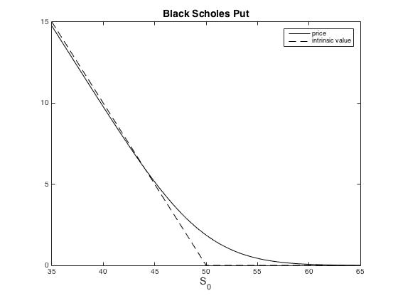
The Black-Scholes put option price for [math]K=50[/math], [math]r=.02[/math], [math]T=3/12[/math], and [math]\sigma=.2[/math] and varying [math]S_0[/math] is shown in Figure.

The Black-Scholes put option price for [math]K=50[/math], [math]r=.02[/math], [math]T=3/12[/math], and [math]\sigma=.2[/math]. Intrinsic value refers to the payoff if exercised now, [math](K-S_0)^+[/math].

Options on Futures and Stocks with Dividends

This section will explain how to compute European derivative prices on stocks with a continuously paying dividend rate, and on future prices. There is some technical issues with stocks paying dividends at a discrete times, but in the case of European options it is merely of matter of considering the future price. Dividends can be an issue in the Black-Scholes theory, particularly because they will determine whether or not Black-Scholes applies for American options (see Section American Options and Optimality of Early Exercise).

Continuous Dividends. Suppose that a European option with payoff [math]\psi(S_T)[/math] is being priced in a market with

[[math]] \begin{eqnarray*} \frac{dS_t}{S_t}&=&(\mu-q)dt+\sigma dW_t\\ dB_t&=&rB_tdt \end{eqnarray*} [[/math]]

where [math]q\geq 0[/math] is the dividend rate. Self-financing in this case has dynamics

[[math]]dV_t = \alpha_tdS_t + r(V_t-\alpha_tS_t)dt+q\alpha_tS_tdt\ .[[/math]]

The replicating strategy from the non-dividend case applies to obtain [math]\alpha_t = \frac{\partial}{\partial s}C(t,S_t)[/math], but the arbitrage argument leads to a different equation,

[[math]] \begin{equation} \label{eq:BSpdeDividends} \left(\frac{\partial}{\partial t}+\frac{\sigma^2s^2}{2}\frac{\partial^2}{\partial s^2}+(r-q)s\frac{\partial}{\partial s}-(r-q)\right)C(t,s) = qC(t,s) \end{equation} [[/math]]

with [math]C(T,s) = \psi(s)[/math]. Equation \eqref{eq:BSpdeDividends} is the Black-Scholes PDE with dividends, and is solved by

[[math]]C(t,S_t) = e^{-q(T-t)}C^1(t,S_t)[[/math]]

where [math]C^1(t,S_t)[/math] solves the Black-Scholes equation of \eqref{eq:BSpde} with [math]r[/math] replaced by [math]r-q[/math]. For example, a European call option on a stock with dividends:

Proposition (Call Option on Stock with Dividends)

[[math]]C(t,S_t) = S_te^{-q(T-t)}N(d_1)-Ke^{-r(T-t)}N(d_2)[[/math]]

where

[[math]] \begin{align*} &d_1 = \frac{\log(S_t/K)+(r-q+.5\sigma^2)(T-t)}{\sigma\sqrt{T-t}} \\ &d_2 = d_1-\sigma\sqrt{T-t}\ . \end{align*} [[/math]]

Futures. Now we turn out attention to futures. Suppose that the spot price on a commodity is given by

[[math]]\frac{dS_t}{S_t}= \mu dt+\sigma dW_t\ .[[/math]]

From arbitrage arguments we know that the future price on [math]S_T[/math] is

[[math]]F_{t,T} \doteq S_te^{r(T-t)}[[/math]]

with [math]F_{T,T}=S_T[/math]. However, [math]S_te^{r(T-t)}[/math] is a martingale under the EMM, and so [math]F_{t,T}[/math] is also a martingale with

[[math]]\frac{dF_{t,T}}{F_{t,T}}=\sigma dW_t^Q\ ,[[/math]]

and the price of a derivative in terms of [math]F_{t,T}[/math] is [math]C(t,F_{t,T}) = e^{-r(T-t)}\widetilde C(t,F_{t,T})[/math] where [math]\widetilde C[/math] satisfies

[[math]] \begin{equation} \label{eq:BSpdeFutures} \left(\frac{\partial}{\partial t}+\frac{\sigma^2x^2}{2}\frac{\partial^2}{\partial x^2}\right)\widetilde C(t,x) = 0 \end{equation} [[/math]]

with [math]\widetilde C(T,x) = \psi(x)[/math]. For example, the call option on the future:

Proposition (Call Option on Future)

[[math]]C(t,F_{t,T}) = e^{-r(T-t)}\left(F_{t,T}N(d_1)-KN(d_2)\right)[[/math]]

where

[[math]] \begin{align*} &d_1 = \frac{\log(F_{t,T}/K)+.5\sigma^2(T-t)}{\sigma\sqrt{T-t}} \\ &d_2 = d_1-\sigma\sqrt{T-t}\ . \end{align*} [[/math]]

The Similarities. Futures contracts certainly have fundamental differences from stocks paying dividends, and vice versa. But the Black-Scholes PDE for pricing options on futures is like that for a stock with dividend rate [math]r[/math]. Alternatively, the future on a dividend paying stock is

[[math]]F_{t,T} = S_te^{(r-q)(T-t)}[[/math]]

which is a non-dividend paying asset and can hence be priced using equation \eqref{eq:BSpdeFutures}.

Discrete-Time Dividends. This interpretation of dividend-paying stocks as futures is useful when dividends are paid at discrete times. Discrete time dividends are described as

[[math]]\log(S_t/S_0) = \left(r-\frac 12 \sigma^2\right)t+\sigma W_t^Q-\sum_{i=0}^{n(t)}\delta_i[[/math]]

where [math]\delta_i[/math] is a proportional dividend rate, and [math]n(t)[/math] is the number of dividends paid up to time [math]t[/math]. The future price of dividend paying stock [math]S_T[/math] is

[[math]]F_{t,T} = S_t\exp\left(\left(r-\frac 12\sigma^2\right)(T-t)-\sum_{i=n(t)+1}^{n(T)}\delta_i\right)\ .[[/math]]

Call option on [math]F_{T,T}[/math] can be priced with equation \eqref{eq:BSpdeFutures}.

General references

Papanicolaou, Andrew (2015). "Introduction to Stochastic Differential Equations (SDEs) for Finance". arXiv:1504.05309 [q-fin.MF].