Ridge Regression

[math] \require{textmacros} \def \bbeta {\bf \beta} \def\fat#1{\mbox{\boldmath$#1$}} \def\reminder#1{\marginpar{\rule[0pt]{1mm}{11pt}}\textbf{#1}} \def\SSigma{\bf \Sigma} \def\ttheta{\bf \theta} \def\aalpha{\bf \alpha} \def\bbeta{\bf \beta} \def\ddelta{\bf \delta} \def\eeta{\bf \eta} \def\llambda{\bf \lambda} \def\ggamma{\bf \gamma} \def\nnu{\bf \nu} \def\vvarepsilon{\bf \varepsilon} \def\mmu{\bf \mu} \def\nnu{\bf \nu} \def\ttau{\bf \tau} \def\SSigma{\bf \Sigma} \def\TTheta{\bf \Theta} \def\XXi{\bf \Xi} \def\PPi{\bf \Pi} \def\GGamma{\bf \Gamma} \def\DDelta{\bf \Delta} \def\ssigma{\bf \sigma} \def\UUpsilon{\bf \Upsilon} \def\PPsi{\bf \Psi} \def\PPhi{\bf \Phi} \def\LLambda{\bf \Lambda} \def\OOmega{\bf \Omega} [/math]

High-throughput techniques measure many characteristics of a single sample simultaneously. The number of characteristics [math]p[/math] measured may easily exceed ten thousand. In most medical studies the number of samples [math]n[/math] involved often falls behind the number of characteristics measured, i.e: [math]p \gt n[/math]. The resulting [math](n \times p)[/math]-dimensional data matrix [math]\mathbf{X}[/math]:

[[math]] \begin{eqnarray*} \mathbf{X} & = & \left( X_{\ast,1} \, | \, \ldots \, | \, X_{\ast,p} \right) \, \, \, = \, \, \, \left( \begin{array}{c} X_{1,\ast} \\ \vdots \\ X_{n,\ast} \end{array} \right) \, \, \, = \, \, \, \left( \begin{array}{ccc} X_{1,1} & \ldots & X_{1,p} \\% \vdots & \ddots & \vdots \\ X_{n,1} & \ldots & X_{n,p} \end{array} \right) \end{eqnarray*} [[/math]]

from such a study contains a larger number of covariates than samples. When [math]p \gt n[/math] the data matrix [math]\mathbf{X}[/math] is said to be high-dimensional, although no formal definition exists.

The information contained in [math]\mathbf{X}[/math] is often used to explain a particular property of the samples involved. In applications in molecular biology [math]\mathbf{X}[/math] may contain microRNA expression data from which the expression levels of a gene are to be described. When the gene's expression levels are denoted by [math]\mathbf{Y} = (Y_{1}, \ldots, Y_n)^{\top}[/math], the aim is to find the linear relation [math]Y_i = \mathbf{X}_{i, \ast} \bbeta[/math] from the data at hand by means of regression analysis. Regression is however frustrated by the high-dimensionality of [math]\mathbf{X}[/math]. We discuss how regression may be modified to accommodate the high-dimensionality of [math]\mathbf{X}[/math].

Linear Regression Review

Consider an experiment in which [math]p[/math] characteristics of [math]n[/math] samples are measured. The data from this experiment are denoted [math]\mathbf{X}[/math], with [math]\mathbf{X}[/math] as above. The matrix [math]\mathbf{X}[/math] is called the design matrix. Additional information of the samples is available in the form of [math]\mathbf{Y}[/math] (also as above). The variable [math]\mathbf{Y}[/math] is generally referred to as the response variable. The aim of regression analysis is to explain [math]\mathbf{Y}[/math] in terms of [math]\mathbf{X}[/math] through a functional relationship like [math]Y_i = f(\mathbf{X}_{i,\ast})[/math]. When no prior knowledge on the form of [math]f(\cdot)[/math] is available, it is common to assume a linear relationship between [math]\mathbf{X}[/math] and [math]\mathbf{Y}[/math]. This assumption gives rise to the linear regression model:

[[math]] \begin{eqnarray} \label{form.linRegressionModel} Y_{i} & = & \mathbf{X}_{i,\ast} \, \bbeta + \varepsilon_i \, \, \, = \, \, \, \beta_1 \, X_{i,1} + \ldots + \beta_{p} \, X_{i, p} + \varepsilon_i. \end{eqnarray} [[/math]]

In model (\ref{form.linRegressionModel}) [math]\bbeta = (\beta_1, \ldots, \beta_p)^{\top}[/math] is the regression parameter. The parameter [math]\beta_j[/math], [math]j=1, \ldots, p[/math], represents the effect size of covariate [math]j[/math] on the response. That is, for each unit change in covariate [math]j[/math] (while keeping the other covariates fixed) the observed change in the response is equal to [math]\beta_j[/math]. The second summand on the right-hand side of the model, [math]\varepsilon_i[/math], is referred to as the error. It represents the part of the response not explained by the functional part [math]\mathbf{X}_{i,\ast} \, \bbeta[/math] of the model (\ref{form.linRegressionModel}). In contrast to the functional part, which is considered to be systematic (i.e. non-random), the error is assumed to be random. Consequently, [math]Y_{i}[/math] need not be equal [math]Y_{i'}[/math] for [math]i \not= i'[/math], even if [math]\mathbf{X}_{i,\ast}= \mathbf{X}_{i',\ast}[/math]. To complete the formulation of model (\ref{form.linRegressionModel}) we need to specify the probability distribution of [math]\varepsilon_i[/math]. It is assumed that [math]\varepsilon_i \sim \mathcal{N}(0, \sigma^2)[/math] and the [math]\varepsilon_{i}[/math] are independent, i.e.:

[[math]] \begin{eqnarray*} \mbox{Cov}(\varepsilon_{i}, \varepsilon_{i'}) & = & \left\{ \begin{array}{lcc} \sigma^2 & \mbox{if} & i = i', \\ 0 & \mbox{if} & i \not= i'. \end{array} \right. \end{eqnarray*} [[/math]]

The randomness of [math]\varepsilon_i[/math] implies that [math]\mathbf{Y}_i[/math] is also a random variable. In particular, [math]\mathbf{Y}_i[/math] is normally distributed, because [math]\varepsilon_i \sim \mathcal{N}(0, \sigma^2)[/math] and [math]\mathbf{X}_{i,\ast} \, \bbeta[/math] is a non-random scalar. To specify the parameters of the distribution of [math]\mathbf{Y}_i[/math] we need to calculate its first two moments. Its expectation equals:

[[math]] \begin{eqnarray*} \mathbb{E}(Y_i) & = & \mathbb{E}(\mathbf{X}_{i, \ast} \, \bbeta) + \mathbb{E}(\varepsilon_i) \, \, \, = \, \, \, \mathbf{X}_{i, \ast} \, \bbeta, \end{eqnarray*} [[/math]]

while its variance is:

[[math]] \begin{eqnarray*} \mbox{Var}(Y_i) & = & \mathbb{E} \{ [Y_i - \mathbb{E}(Y_i)]^2 \} \qquad \qquad \qquad \qquad \qquad \quad = \, \, \, \mathbb{E} ( Y_i^2 ) - [\mathbb{E}(Y_i)]^2 \\ & = & \mathbb{E} [ ( \mathbf{X}_{i, \ast} \, \bbeta)^2 + 2 \varepsilon_i \mathbf{X}_{i, \ast} \, \bbeta + \varepsilon_i^2 ] - ( \mathbf{X}_{i, \ast} \, \bbeta)^2 \, \, \, = \, \, \, \mathbb{E}(\varepsilon_i^2 ) \\ & = & \mbox{Var}(\varepsilon_i ) \qquad \qquad \qquad \qquad \qquad \qquad \qquad \quad \, \, = \, \, \, \sigma^2. \end{eqnarray*} [[/math]]

Hence, [math]Y_i \sim \mathcal{N}( \mathbf{X}_{i, \ast} \, \bbeta, \sigma^2)[/math]. This formulation (in terms of the normal distribution) is equivalent to the formulation of model (\ref{form.linRegressionModel}), as both capture the assumptions involved: the linearity of the functional part and the normality of the error.

Model (\ref{form.linRegressionModel}) is often written in a more condensed matrix form:

[[math]] \begin{eqnarray} \mathbf{Y} & = & \mathbf{X} \, \bbeta + \vvarepsilon, \label{form.linRegressionModelinMatrix} \end{eqnarray} [[/math]]

where [math]\vvarepsilon = (\varepsilon_1, \varepsilon_2, \ldots, \varepsilon_n)^{\top}[/math] and distributed as [math]\vvarepsilon \sim \mathcal{N}(\mathbf{0}_{p}, \sigma^2 \mathbf{I}_{nn})[/math]. As above model (\ref{form.linRegressionModelinMatrix}) can be expressed as a multivariate normal distribution: [math]\mathbf{Y} \sim \mathcal{N}(\mathbf{X} \, \bbeta, \sigma^2 \mathbf{I}_{nn})[/math].

Model (\ref{form.linRegressionModelinMatrix}) is a so-called hierarchical model. This terminology emphasizes that [math]\mathbf{X}[/math] and [math]\mathbf{Y}[/math] are not on a par, they play different roles in the model. The former is used to explain the latter. In model (\ref{form.linRegressionModel}) [math]\mathbf{X}[/math] is referred as the explanatory or independent variable, while the variable [math]\mathbf{Y}[/math] is generally referred to as the response or dependent variable.

The covariates, the columns of [math]\mathbf{X}[/math], may themselves be random. To apply the linear model they are temporarily assumed fixed. The linear regression model is then to be interpreted as [math]\mathbf{Y} \, | \, \mathbf{X} \sim \mathcal{N}(\mathbf{X} \, \bbeta, \sigma^2 \mathbf{I}_{nn})[/math]

The linear regression model (\ref{form.linRegressionModel}) involves the unknown parameters: [math]\bbeta[/math] and [math]\sigma^2[/math], which need to be learned from the data. The parameters of the regression model, [math]\bbeta[/math] and [math]\sigma^2[/math] are estimated by means of likelihood maximization. Recall that [math]Y_i \sim \mathcal{N}( \mathbf{X}_{i,\ast} \, \bbeta, \sigma^2)[/math] with corresponding density: [math] f_{Y_i}(y_i) = (2 \, \pi \, \sigma^2)^{-1/2} \, \exp[ - (y_i - \mathbf{X}_{i\ast} \, \bbeta)^2 / 2 \sigma^2 ][/math]. The likelihood thus is:

[[math]] \begin{eqnarray*} L(\mathbf{Y}, \mathbf{X}; \bbeta, \sigma^2) & = & \prod_{i=1}^n (\sqrt{2 \, \pi} \, \sigma)^{-1} \, \exp[ - (Y_i - \mathbf{X}_{i, \ast} \, \bbeta)^2 / 2 \sigma^2 ], \end{eqnarray*} [[/math]]

in which the independence of the observations has been used. Because of the concavity of the logarithm, the maximization of the likelihood coincides with the maximum of the logarithm of the likelihood (called the log-likelihood). Hence, to obtain maximum likelihood (ML) estimates of the parameter it is equivalent to find the maximum of the log-likelihood. The log-likelihood is:

[[math]] \begin{eqnarray*} \mathcal{L}(\mathbf{Y}, \mathbf{X}; \bbeta, \sigma^2) & = & \log[ L(\mathbf{Y}, \mathbf{X}; \bbeta, \sigma^2) ] \, \, \, = \, \, \, % \log \Big[ \prod_{i=1}^n f_{Y_i}(y_i) \Big] -n \, \log(\sqrt{2 \, \pi} \, \sigma) - \tfrac{1}{2} \sigma^{-2} \sum\nolimits_{i=1}^n (y_i - \mathbf{X}_{i, \ast} \, \bbeta)^2. \end{eqnarray*} [[/math]]

After noting that [math]\sum_{i=1}^n (Y_i - \mathbf{X}_{i, \ast} \, \bbeta)^2 = \| \mathbf{Y} - \mathbf{X} \, \bbeta \|^2_2 \, \, \, = \, \, \, (\mathbf{Y} - \mathbf{X} \, \bbeta)^{\top} \, (\mathbf{Y} - \mathbf{X} \, \bbeta)[/math], the log-likelihood can be written as:

[[math]] \begin{eqnarray*} \mathcal{L}(\mathbf{Y}, \mathbf{X}; \bbeta, \sigma^2) & = & -n \, \log(\sqrt{2 \, \pi} \, \sigma) - \tfrac{1}{2} \sigma^{-2} \, \| \mathbf{Y} - \mathbf{X} \, \bbeta \|^2_2. \end{eqnarray*} [[/math]]

In order to find the maximum of the log-likelihood, take its derivate with respect to [math]\bbeta[/math]:

[[math]] \begin{eqnarray*} \frac{\partial }{\partial \, \beta} \mathcal{L}(\mathbf{Y}, \mathbf{X}; \bbeta, \sigma^2) & = & - \tfrac{1}{2} \sigma^{-2} \, \frac{\partial }{\partial \, \beta} \| \mathbf{Y} - \mathbf{X} \, \bbeta \|^2_2 \, \, \, = \, \, \, \tfrac{1}{2} \sigma^{-2} \, \mathbf{X}^{\top} (\mathbf{Y} - \mathbf{X} \, \bbeta). \end{eqnarray*} [[/math]]

Equate this derivative to zero gives the estimating equation for [math]\bbeta[/math]:

[[math]] \begin{eqnarray} \label{form.normalEquation} \mathbf{X}^{\top} \mathbf{X} \, \bbeta & = & \mathbf{X}^{\top} \mathbf{Y}. \end{eqnarray} [[/math]]

Equation (\ref{form.normalEquation}) is called to the normal equation. Pre-multiplication of both sides of the normal equation by [math](\mathbf{X}^{\top} \mathbf{X})^{-1}[/math] now yields the ML estimator of the regression parameter: [math]\hat{\bbeta} = (\mathbf{X}^{\top} \mathbf{X})^{-1} \, \mathbf{X}^{\top} \mathbf{Y}[/math], in which it is assumed that [math](\mathbf{X}^{\top} \mathbf{X})^{-1}[/math] is well-defined.

Along the same lines one obtains the ML estimator of the residual variance. Take the partial derivative of the loglikelihood with respect to [math]\sigma^2[/math]:

[[math]] \begin{eqnarray*} \frac{\partial }{\partial \, \sigma} \mathcal{L}(\mathbf{Y}, \mathbf{X}; \bbeta, \sigma^2) & = & - \sigma^{-1} + \sigma^{-3} \| \mathbf{Y} - \mathbf{X} \, \bbeta \|^2_2. \end{eqnarray*} [[/math]]

Equate the right-hand side to zero and solve for [math]\sigma^2[/math] to find [math]\hat{\sigma}^2 = n^{-1} \| \mathbf{Y} - \mathbf{X} \, \bbeta \|^2_2[/math]. In this expression [math]\bbeta[/math] is unknown and the ML estimate of [math]\bbeta[/math] is plugged-in.

With explicit expressions of the ML estimators at hand, we can study their properties. The expectation of the ML estimator of the regression parameter [math]\bbeta[/math] is:

[[math]] \begin{eqnarray*} \mathbb{E}(\hat{\bbeta}) & = & \mathbb{E}[ (\mathbf{X}^{\top} \mathbf{X})^{-1} \, \mathbf{X}^{\top} \mathbf{Y}] \, \, \, = \, \, \, (\mathbf{X}^{\top} \mathbf{X})^{-1} \, \mathbf{X}^{\top} \mathbb{E}( \mathbf{Y}) \, \, \, = \, \, \, (\mathbf{X}^{\top} \mathbf{X})^{-1} \, \mathbf{X}^{\top} \mathbf{X} \, \bbeta \, \, \, \, \, = \, \, \, \bbeta. \end{eqnarray*} [[/math]]

Hence, the ML estimator of the regression coefficients is unbiased.

The variance of the ML estimator of [math]\bbeta[/math] is:

[[math]] \begin{eqnarray*} \mbox{Var}(\hat{\bbeta}) & = & \mathbb{E} \{ [\hat{\bbeta} - \mathbb{E}(\hat{\bbeta})] [\hat{\bbeta} - \mathbb{E}(\hat{\bbeta})]^{\top} \} \\ & = & \mathbb{E} \{ [(\mathbf{X}^{\top} \mathbf{X})^{-1} \, \mathbf{X}^{\top} \mathbf{Y} - \bbeta] \, [(\mathbf{X}^{\top} \mathbf{X})^{-1} \, \mathbf{X}^{\top} \mathbf{Y} - \bbeta]^{\top} \} \\ & = & (\mathbf{X}^{\top} \mathbf{X})^{-1} \, \mathbf{X}^{\top} \, \mathbb{E} \{ \mathbf{Y} \, \mathbf{Y}^{\top} \} \, \mathbf{X} \, (\mathbf{X}^{\top} \mathbf{X})^{-1} - \bbeta \, \bbeta^{\top} \\ & = & (\mathbf{X}^{\top} \mathbf{X})^{-1} \, \mathbf{X}^{\top} \, \{ \mathbf{X} \, \bbeta \, \bbeta^{\top} \, \mathbf{X}^{\top} + \SSigma \} \, \mathbf{X} \, (\mathbf{X}^{\top} \mathbf{X})^{-1} - \bbeta \, \bbeta^{\top} \\ & = & \bbeta \, \bbeta^{\top} + \sigma^2 \, (\mathbf{X}^{\top} \mathbf{X})^{-1} - \bbeta \, \bbeta^{\top} \\ & = & \sigma^2 \, (\mathbf{X}^{\top} \mathbf{X})^{-1}, \end{eqnarray*} [[/math]]

in which we have used that [math]\mathbb{E} (\mathbf{Y} \mathbf{Y}^{\top}) = \mathbf{X} \, \bbeta \, \bbeta^{\top} \, \mathbf{X}^{\top} + \sigma^2 \, \mathbf{I}_{nn}[/math]. From [math]\mbox{Var}(\hat{\bbeta}) = \sigma^2 \, (\mathbf{X}^{\top} \mathbf{X})^{-1}[/math], one obtains an estimate of the variance of the estimator of the [math]j[/math]-th regression coefficient: [math]\hat{\sigma}^2 (\hat{\beta}_j ) = \hat{\sigma}^2 \sqrt{ [(\mathbf{X}^{\top} \mathbf{X})^{-1}]_{jj} }[/math]. This may be used to construct a confidence interval for the estimates or test the hypothesis [math]H_0: \beta_j = 0[/math]. In the latter [math]\hat{\sigma}^2[/math] should not be the maximum likelihood estimator, as it is biased. It is then to be replaced by the residual sum-of-squares divided by [math]n-p[/math] rather than [math]n[/math].

The prediction of [math]Y_i[/math], denoted [math]\widehat{Y}_i[/math], is the expected value of [math]Y_i[/math] according the linear regression model (with its parameters replaced by their estimates). The prediction of [math]Y_i[/math] thus equals [math]\mathbb{E}(Y_i; \hat{\bbeta}, \hat{\sigma}^2) = \mathbf{X}_{i, \ast} \hat{\bbeta}[/math]. In matrix notation the prediction is:

[[math]] \begin{eqnarray*} \widehat{\mathbf{Y}} & = & \mathbf{X} \, \hat{\bbeta} \, \, \, = \, \, \, \mathbf{X} \, (\mathbf{X}^{\top} \mathbf{X})^{-1} \mathbf{X}^{\top} \mathbf{Y} \, \, \, := \, \, \, \mathbf{H} \mathbf{Y}, \end{eqnarray*} [[/math]]

where [math]\mathbf{H}[/math] is the hat matrix, as it ‘puts the hat’ on [math]\mathbf{Y}[/math]. Note that the hat matrix is a projection matrix, i.e. [math]\mathbf{H}^2 = \mathbf{H}[/math] for

[[math]] \begin{eqnarray*} \mathbf{H}^2 & = & \mathbf{X} \, (\mathbf{X}^{\top} \mathbf{X})^{-1} \mathbf{X}^{\top} \mathbf{X} \, (\mathbf{X}^{\top} \mathbf{X})^{-1} \mathbf{X}^{\top} \, \, \, = \, \, \, \mathbf{X} \, (\mathbf{X}^{\top} \mathbf{X})^{-1} \mathbf{X}^{\top}. \end{eqnarray*} [[/math]]

Thus, the prediction [math]\widehat{\mathbf{Y}}[/math] is an orthogonal projection of [math]\mathbf{Y}[/math] onto the space spanned by the columns of [math]\mathbf{X}[/math].

With [math]\widehat{\bbeta}[/math] available, an estimate of the errors [math]\hat{\varepsilon}_i[/math], dubbed the residuals are obtained via:

[[math]] \begin{eqnarray*} \hat{\vvarepsilon} & = & \mathbf{Y} - \widehat{\mathbf{Y}} \, \, \, = \, \, \, \mathbf{Y} - \mathbf{X} \, \hat{\bbeta} \, \, \, = \, \, \, \mathbf{Y} - \mathbf{X} \, (\mathbf{X}^{\top} \mathbf{X})^{-1} \mathbf{X}^{\top} \mathbf{Y} \, \, \, = \, \, \, [ \mathbf{I} - \mathbf{X} \, (\mathbf{X}^{\top} \mathbf{X})^{-1} \mathbf{X}^{\top} ] \, \mathbf{Y}. \end{eqnarray*} [[/math]]

Thus, the residuals are a projection of [math]\mathbf{Y}[/math] onto the orthogonal complement of the space spanned by the columns of [math]\mathbf{X}[/math]. The residuals are to be used in diagnostics, e.g. checking of the normality assumption by means of a normal probability plot.

The ridge regression estimator

If the design matrix is high-dimensional, the covariates (the columns of [math]\mathbf{X}[/math]) are super-collinear. Recall collinearity in regression analysis refers to the event of two (or multiple) covariates being strongly linearly related. Consequently, the space spanned by super-collinear covariates is then a lower-dimensional subspace of the parameter space. If the design matrix [math]\mathbf{X}[/math], which contains the collinear covariates as columns, is (close to) rank deficient, it is (almost) impossible to separate the contribution of the individual covariates. The uncertainty with respect to the covariate responsible for the variation explained in [math]\mathbf{Y}[/math] is often reflected in the fit of the linear regression model to data by a large error of the estimates of the regression parameters corresponding to the collinear covariates and, consequently, usually accompanied by large values of the estimates.

Example (Super-collinearity)

Consider the design matrix:

[[math]] \begin{eqnarray*} \mathbf{X} & = & \left( \begin{array}{rrr} 1 & -1 & 2 \\ 1 & 0 & 1 \\ 1 & 2 & -1 \\ 1 & 1 & 0 \end{array} \right) \end{eqnarray*} [[/math]]

The columns of [math]\mathbf{X}[/math] are linearly dependent: the first column is the row-wise sum of the other two columns. The rank (more correct, the column rank) of a matrix is the dimension of space spanned by the column vectors. Hence, the rank of [math]\mathbf{X}[/math] is equal to the number of linearly independent columns: [math]\mbox{rank}(\mathbf{X}) = 2[/math].

Super-collinearity of an [math](n \times p)[/math]-dimensional design matrix [math]\mathbf{X}[/math] implies\footnote{If the (column) rank of [math]\mathbf{X}[/math] is smaller than [math]p[/math], there exists a non-trivial [math]\mathbf{v} \in \mathbb{R}^p[/math] such that [math]\mathbf{X} \mathbf{v} = \mathbf{0}_{p}[/math]. Multiplication of this inequality by [math]\mathbf{X}^{\top}[/math] yields [math]\mathbf{X}^{\top} \mathbf{X} \mathbf{v} = \mathbf{0}_{p}[/math]. As [math]\mathbf{v} \not= \mathbf{0}_{p}[/math], this implies that [math]\mathbf{X}^{\top} \mathbf{X}[/math] is not invertible.} that the rank of the [math](p \times p)[/math]-dimensional matrix [math]\mathbf{X}^{\top} \mathbf{X}[/math] is smaller than [math]p[/math], and, consequently, it is singular. A square matrix that does not have an inverse is called singular. A matrix [math]\mathbf{A}[/math] is singular if and only if its determinant is zero: [math]\mbox{det}(\mathbf{A}) = 0[/math].

Example (Singularity)

Consider the matrix [math]\mathbf{A}[/math] given by:

[[math]] \begin{eqnarray*} \mathbf{A} & = & \left( \begin{array}{rr} 1 & 2 \\ 2 & 4 \end{array} \right) \end{eqnarray*} [[/math]]

Clearly, [math]\mbox{det}(\mathbf{A}) = a_{11} a_{22} - a_{12} a_{21} = 1 \times 4 - 2 \times 2 = 0[/math]. Hence, [math]\mathbf{A}[/math] is singular and its inverse is undefined.

As [math]\mbox{det}(\mathbf{A})[/math] is equal to the product of the eigenvalues [math]\nu_j[/math] of [math]\mathbf{A}[/math], the matrix [math]\mathbf{A}[/math] is singular if one (or more) of the eigenvalues of [math]\mathbf{A}[/math] is zero. To see this, consider the spectral decomposition of [math]\mathbf{A}[/math]: [math]\mathbf{A} = \sum_{j=1}^p \nu_j \, \mathbf{v}_j \, \mathbf{v}_j^{\top}[/math], where [math]\mathbf{v}_j[/math] is the eigenvector corresponding to [math]\nu_j[/math]. To obtain the inverse of [math]\mathbf{A}[/math] it requires to take the reciprocal of the eigenvalues: [math]\mathbf{A}^{-1} = \sum_{j=1}^p \nu_j^{-1} \, \mathbf{v}_j \, \mathbf{v}_j^{\top}[/math]. The right-hand side is undefined if [math]\nu_j =0[/math] for any [math]j[/math].

Example (Singularity, continued)

Revisit Example. Matrix [math]\mathbf{A}[/math] has eigenvalues [math]\nu_1 =5[/math] and [math]\nu_2=0[/math]. According to the spectral decomposition, the inverse of [math]\mathbf{A}[/math] is: [math]\mathbf{A}^{-1} = \tfrac{1}{5} \, \mathbf{v}_1 \, \mathbf{v}_1^{\top} + \tfrac{1}{0} \, \mathbf{v}_2 \, \mathbf{v}_2^{\top}[/math]. This expression is undefined as we divide by zero in the second summand on the right-hand side.

In summary, the columns of a high-dimensional design matrix [math]\mathbf{X}[/math] are linearly dependent and this super-collinearity causes [math]\mathbf{X}^{\top} \mathbf{X}[/math] to be singular. Now recall the ML estimator of the parameter of the linear regression model: [math]\hat{\bbeta} = (\mathbf{X}^{\top} \mathbf{X})^{-1} \mathbf{X}^{\top} \mathbf{Y}[/math]. This estimator is only well-defined if [math](\mathbf{X}^{\top} \mathbf{X})^{-1}[/math] exits. Hence, when [math]\mathbf{X}[/math] is high-dimensional the regression parameter [math]\bbeta[/math] cannot be estimated.

Above only the practical consequence of high-dimensionality is presented: the expression [math]( \mathbf{X}^{\top} \mathbf{X})^{-1} \mathbf{X}^{\top} \mathbf{Y}[/math] cannot be evaluated numerically. But the problem arising from the high-dimensionality of the data is more fundamental. To appreciate this, consider the normal equations: [math]\mathbf{X}^{\top} \mathbf{X} \bbeta = \mathbf{X}^{\top} \mathbf{Y}[/math]. The matrix [math]\mathbf{X}^{\top} \mathbf{X}[/math] is of rank [math]n[/math], while [math]\bbeta[/math] is a vector of length [math]p[/math]. Hence, while there are [math]p[/math] unknowns, the system of linear equations from which these are to be solved effectively comprises [math]n[/math] degrees of freedom. If [math]p \gt n[/math], the vector [math]\bbeta[/math] cannot uniquely be determined from this system of equations. To make this more specific let [math]\mathcal{U}[/math] be the [math]n[/math]-dimensional space spanned by the columns of [math]\mathbf{X}[/math] and the [math]p-n[/math]-dimensional space [math]\mathcal{V}[/math] be orthogonal complement of [math]\mathcal{U}[/math], i.e. [math]\mathcal{V} = \mathcal{U}^{\perp}[/math]. Then, [math]\mathbf{X} \mathbf{v} = \mathbf{0}_{p}[/math] for all [math]\mathbf{v} \in \mathcal{V}[/math]. So, [math]\mathcal{V}[/math] is the non-trivial null space of [math]\mathbf{X}[/math]. Consequently, as [math]\mathbf{X}^{\top} \mathbf{X} \mathbf{v} = \mathbf{X}^{\top} \mathbf{0}_{p} = \mathbf{0}_{n}[/math], the solution of the normal equations is:

[[math]] \begin{eqnarray*} \hat{\bbeta} & = & ( \mathbf{X}^{\top} \mathbf{X})^{+} \mathbf{X}^{\top} \mathbf{Y} + \mathbf{v} \qquad \mbox{for all } \mathbf{v} \in \mathcal{V}, \end{eqnarray*} [[/math]]

where [math]\mathbf{A}^{+}[/math] denotes the Moore-Penrose inverse of the matrix [math]\mathbf{A}[/math] (adopting the notation of ). For a square symmetric matrix, the generalized inverse is defined as:

[[math]] \begin{eqnarray*} \mathbf{A}^{+} & = & \sum\nolimits_{j=1}^p \nu_j^{-1} \, I_{\{ \nu_j \not= 0 \} } \, \mathbf{v}_j \, \mathbf{v}_j^{\top}, \end{eqnarray*} [[/math]]

where [math]\mathbf{v}_j[/math] are the eigenvectors of [math]\mathbf{A}[/math] (and are not -- necessarily -- an element of [math]\mathcal{V}[/math]). The solution of the normal equations is thus only determined up to an element from a non-trivial space [math]\mathcal{V}[/math], and there is no unique estimator of the regression parameter. % With this mind, the ridge estimator can then be thought of as altering the normal equations provide a unique solution for [math]\bbeta[/math].

To arrive at a unique regression estimator for studies with rank deficient design matrices, the minimum least squares estimator may be employed.

Definition

The minimum least squares estimator of regression parameter minimizes the sum-of-squares criterion and is of minimum length. Formally, [math]\hat{\bbeta}_{\mbox{{\tiny MLS}}} = \arg \min_{\bbeta \in \mathbb{R}^p} \| \mathbf{Y} - \mathbf{X} \bbeta \|_2^2[/math] such that [math]\| \hat{\bbeta}_{\mbox{{\tiny MLS}}} \|_2^2 \lt \| \bbeta \|_2^2[/math] for all [math]\bbeta[/math] that minimize [math]\| \mathbf{Y} - \mathbf{X} \bbeta \|_2^2[/math].

If [math]\mathbf{X}[/math] is of full rank, the minimum least squares regression estimator coincides with the least squares/maximum likelihood one as the latter is a unique minimizer of the sum-of-squares criterion and, thereby, automatically also the minimizer of minimum length. When [math]\mathbf{X}[/math] is rank deficient, [math]\hat{\bbeta}_{\mbox{{\tiny MLS}}} = (\mathbf{X}^{\top} \mathbf{X})^+ \mathbf{X}^{\top} \mathbf{Y}[/math]. To see this recall from above that [math]\| \mathbf{Y} - \mathbf{X} \bbeta \|_2^2[/math] is minimized by [math](\mathbf{X}^{\top} \mathbf{X})^+ \mathbf{X}^{\top} \mathbf{Y} + \mathbf{v}[/math] for all [math]\mathbf{v} \in V[/math]. The length of these minimizers is:

[[math]] \begin{eqnarray*} \| (\mathbf{X}^{\top} \mathbf{X})^+ \mathbf{X}^{\top} \mathbf{Y} + \mathbf{v} \|_2^2 & = & \| (\mathbf{X}^{\top} \mathbf{X})^+ \mathbf{X}^{\top} \mathbf{Y} \|_2^2 + 2 \mathbf{Y}^{\top} \mathbf{X} (\mathbf{X}^{\top} \mathbf{X})^+ \mathbf{v} + \| \mathbf{v} \|_2^2, \end{eqnarray*} [[/math]]

which, by the orthogonality of [math]V[/math] and the space spanned by the columns of [math]\mathbf{X}[/math], equals [math]\| (\mathbf{X}^{\top} \mathbf{X})^+ \mathbf{X}^{\top} \mathbf{Y} \|_2^2 + \| \mathbf{v} \|_2^2[/math]. Clearly, any nontrivial [math]\mathbf{v}[/math], i.e. [math]\mathbf{v} \not= \mathbf{0}_p[/math], results in [math]\| (\mathbf{X}^{\top} \mathbf{X})^+ \mathbf{X}^{\top} \mathbf{Y} \|_2^2 + \| \mathbf{v} \|_2^2 \gt \| (\mathbf{X}^{\top} \mathbf{X})^+ \mathbf{X}^{\top} \mathbf{Y} \|_2^2[/math] and, thus, [math]\hat{\bbeta}_{\mbox{{\tiny MLS}}} = (\mathbf{X}^{\top} \mathbf{X})^+ \mathbf{X}^{\top} \mathbf{Y}[/math].

An alternative (and related) estimator of the regression parameter [math]\bbeta[/math] that avoids the use of the Moore-Penrose inverse and is able to deal with (super)-collinearity among the columns of the design matrix is the ridge regression estimator proposed by . It essentially comprises of an ad-hoc fix to resolve the (almost) singularity of [math]\mathbf{X}^{\top} \mathbf{X}[/math]. propose to simply replace [math]\mathbf{X}^{\top} \mathbf{X}[/math] by [math]\mathbf{X}^{\top} \mathbf{X} + \lambda \mathbf{I}_{pp}[/math] with [math]\lambda \in [0, \infty)[/math]. The scalar [math]\lambda[/math] is a tuning parameter, henceforth called the penalty parameter for reasons that will become clear later. The ad-hoc fix solves the singularity as it adds a positive matrix, [math]\lambda \mathbf{I}_{pp}[/math], to a positive semi-definite one, [math]\mathbf{X}^{\top} \mathbf{X}[/math], making the total a positive definite matrix (Lemma 14.2.4 of ), which is invertible.

Example (Super-collinearity, continued)

Recall the super-collinear design matrix [math]\mathbf{X}[/math] of Example. Then, for (say) [math]\lambda = 1[/math]:

[[math]] \begin{eqnarray*} \mathbf{X}^{\top} \mathbf{X} + \lambda \mathbf{I}_{pp} & = & \left( \begin{array}{rrr} 5 & 2 & 2 \\ 2 & 7 & -4 \\ 2 & -4 & 7 \end{array} \right). \end{eqnarray*} [[/math]]

The eigenvalues of this matrix are 11, 7, and 1. Hence, [math]\mathbf{X}^{\top} \mathbf{X} + \lambda \mathbf{I}_{pp}[/math] has no zero eigenvalue and its inverse is well-defined.

With the ad-hoc fix for the singularity of [math]\mathbf{X}^{\top} \mathbf{X}[/math], proceed to define the ridge regression estimator:

[[math]] \begin{eqnarray} \label{form.ridgeRegressionEstimator} \hat{\bbeta}(\lambda) & = & (\mathbf{X}^{\top} \mathbf{X} + \lambda \mathbf{I}_{pp})^{-1} \mathbf{X}^{\top} \mathbf{Y}, \end{eqnarray} [[/math]]

for [math]\lambda \in [0, \infty)[/math]. Clearly, this is for [math]\lambda[/math] strictly positive (Question discussed the consequences of a negative values of [math]\lambda[/math]) a well-defined estimator, even if [math]\mathbf{X}[/math] is high-dimensional. However, each choice of [math]\lambda[/math] leads to a different ridge regression estimate. The set of all ridge regression estimates [math]\{ \hat{\bbeta}(\lambda) \, : \, \lambda \in [0, \infty) \}[/math] is called the solution or regularization path of the ridge estimator.

Example (Super-collinearity, continued)

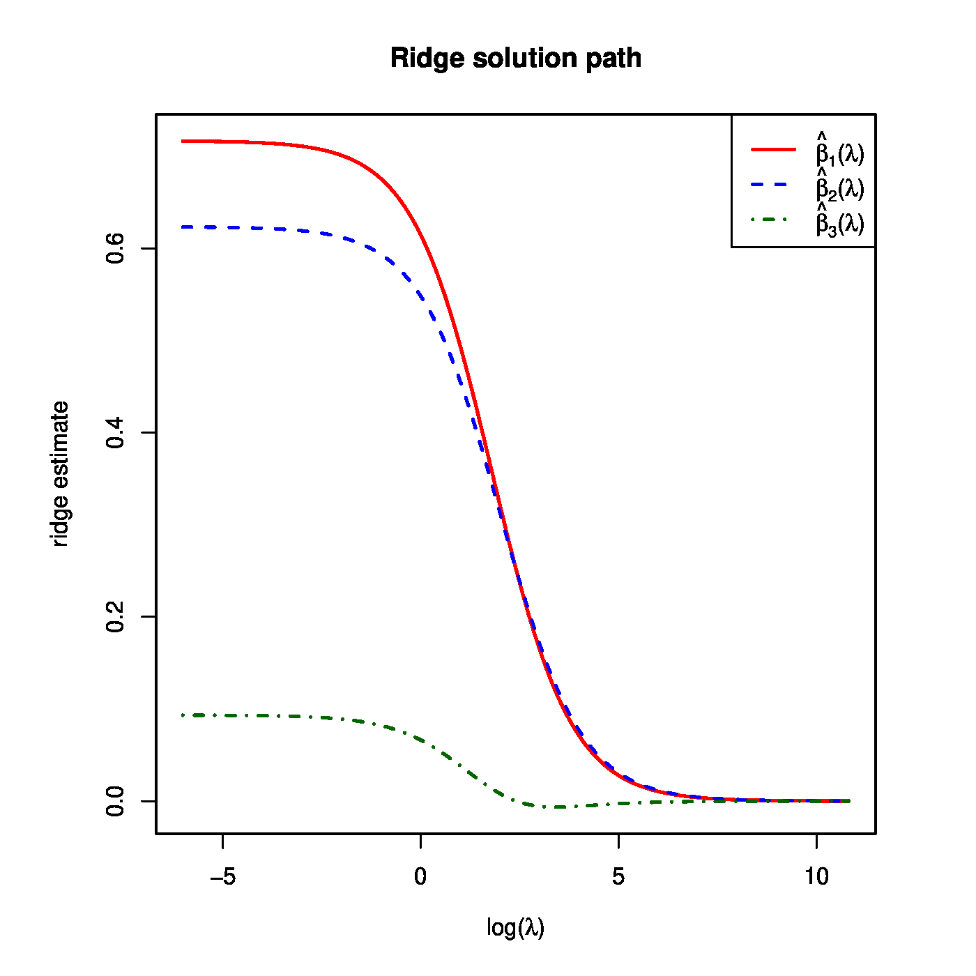
Recall the super-collinear design matrix [math]\mathbf{X}[/math] of Example. Suppose that the corresponding response vector is [math]\mathbf{Y} = (1.3, -0.5, 2.6, 0.9)^{\top}[/math]. The ridge regression estimates for, e.g. [math]\lambda = 1, 2[/math], and [math]10[/math] are then: [math]\hat{\bbeta}(1) = (0.614, 0.548, 0.066)^{\top}[/math], [math]\hat{\bbeta}(2) = (0.537, 0.490, 0.048)^{\top}[/math], and [math]\hat{\bbeta}(10) = (0.269, 0.267, 0.002)^{\top}[/math]. The full solution path of the ridge estimator is shown in the left-hand side panel of Figure.

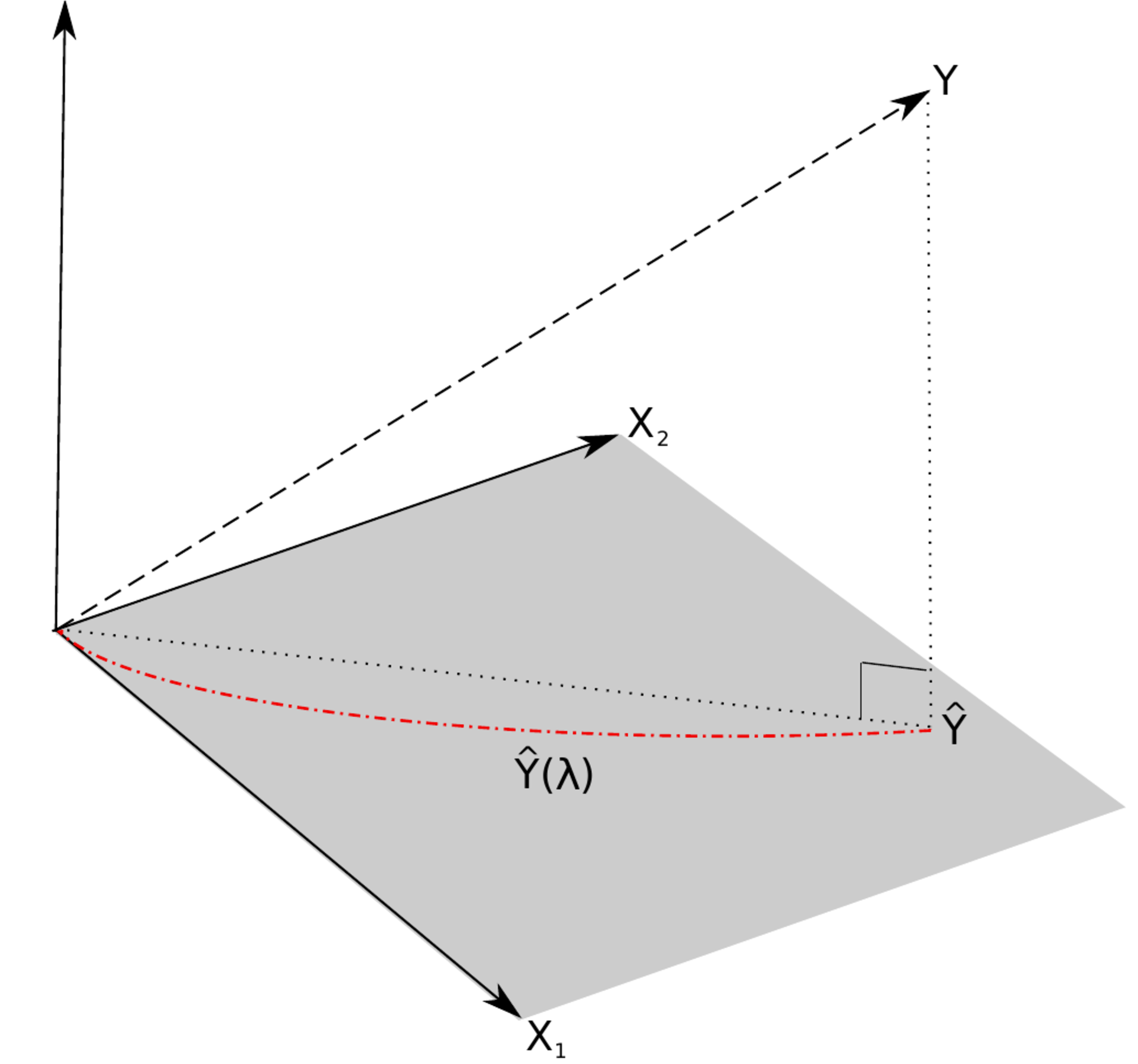
Left panel: the regularization path of the ridge estimator for the data of Example. Right panel: the ‘maximum likelihood fit’ [math]\widehat{Y}[/math] and the ‘ridge fit’ [math]\widehat{Y}(\lambda)[/math] (the dashed-dotted red line) to the observation [math]Y[/math] in the (hyper)plane spanned by the covariates.

Low-dimensionally, when [math]\mathbf{X}^{\top} \mathbf{X}[/math] is of full rank, the ridge regression estimator is linearly related to its maximum likelihood counterpart. To see this define the linear operator [math]\mathbf{W}_{\lambda} = (\mathbf{X}^{\top} \mathbf{X} + \lambda \mathbf{I}_{pp})^{-1} \mathbf{X}^{\top} \mathbf{X}[/math]. The ridge estimator [math]\hat{\bbeta}(\lambda)[/math] can then be expressed as [math]\mathbf{W}_{\lambda} \hat{\bbeta}[/math] for:

[[math]] \begin{eqnarray*} \mathbf{W}_{\lambda} \hat{\bbeta} & = & \mathbf{W}_{\lambda} (\mathbf{X}^{\top} \mathbf{X})^{-1} \mathbf{X}^{\top} \mathbf{Y} \\ & = & ( \mathbf{X}^{\top} \mathbf{X} + \lambda \mathbf{I}_{pp} )^{-1} \mathbf{X}^{\top} \mathbf{X} (\mathbf{X}^{\top} \mathbf{X})^{-1} \mathbf{X}^{\top} \mathbf{Y} \\ & = & ( \mathbf{X}^{\top} \mathbf{X} + \lambda \mathbf{I}_{pp} )^{-1} \mathbf{X}^{\top} \mathbf{Y} \\ & = & \hat{\bbeta}(\lambda). \end{eqnarray*} [[/math]]

The linear operator [math]\mathbf{W}_{\lambda}[/math] thus transforms the maximum likelihood estimator of the regression parameter into its ridge regularized counterpart. High-dimensionally, no such linear relation between the ridge and the minimum least squares regression estimators exists (see Exercise).

With an estimate of the regression parameter [math]\bbeta[/math] available one can define the fit. For the ridge regression estimator the fit is defined analogous to the ML case:

[[math]] \begin{eqnarray*} \widehat{\mathbf{Y}}(\lambda) & = & \mathbf{X} \hat{\bbeta}(\lambda) \, \, \, = \, \, \, \mathbf{X} (\mathbf{X}^{\top} \mathbf{X} + \lambda \mathbf{I}_{pp})^{-1} \mathbf{X}^{\top} \mathbf{Y} \, \, \, := \, \, \, \mathbf{H}(\lambda) \mathbf{Y}. \end{eqnarray*} [[/math]]

For the ML regression estimator the fit could be understood as a projection of [math]\mathbf{Y}[/math] onto the subspace spanned by the columns of [math]\mathbf{X}[/math]. This is depicted in the right panel of Figure, where [math]\widehat{Y}[/math] is the projection of the observation [math]Y[/math] onto the covariate space. The projected observation [math]\widehat{Y}[/math] is orthogonal to the residual [math]\varepsilon = Y - \widehat{Y}[/math]. This means the fit is the point in the covariate space closest to the observation. Put differently, the covariate space does not contain a point that is better (in some sense) in explaining the observation. Compare this to the ‘ridge fit’ which is plotted as a dashed-dotted red line in the right panel of Figure. The ‘ridge fit’ is a line, parameterized by [math]\{ \lambda : \lambda \in \mathbb{R}_{\geq 0} \}[/math], where each point on this line matches to the corresponding intersection of the regularization path [math]\hat{\bbeta}(\lambda)[/math] and the vertical line [math]x=\lambda[/math]. The ‘ridge fit’ [math]\widehat{Y}(\lambda)[/math] runs from the ML fit [math]\widehat{Y} = \widehat{Y} (0)[/math] to an intercept-only fit in which the covariates do not contribute to the explanation of the observation. From the figure it is obvious that for any [math]\lambda \gt 0[/math] the ‘ridge fit’ [math]\widehat{Y}(\lambda)[/math] is not orthogonal to the observation [math]Y[/math]. In other words, the ‘ridge residuals’ [math]Y - \widehat{Y}(\lambda)[/math] are not orthogonal to the fit [math]\widehat{Y}(\lambda)[/math] (confer Exercise ). Hence, the ad-hoc fix of the ridge regression estimator resolves the non-evaluation of the estimator in the face of super-collinearity but yields a ‘ridge fit’ that is not optimal in explaining the observation. Mathematically, this is due to the fact that the fit [math]\widehat{Y}(\lambda)[/math] corresponding to the ridge regression estimator is not a projection of [math]Y[/math] onto the covariate space (confer Exercise).

Moments

The first two moments of the ridge regression estimator are derived. Next the performance of the ridge regression estimator is studied in terms of the mean squared error, which combines the first two moments.

Expectation

The left panel of Figure shows ridge estimates of the regression parameters converging to zero as the penalty parameter tends to infinity. This behaviour of the ridge estimator does not depend on the specifics of the data set. To see this study the expectation of the ridge estimator:

[[math]] \begin{eqnarray*} \mathbb{E} \big[ \hat{\bbeta}(\lambda) \big] & = & \mathbb{E} \big[ (\mathbf{X}^{\top} \mathbf{X} + \lambda \mathbf{I}_{pp})^{-1} \mathbf{X}^{\top} \mathbf{Y} \big] \, \, \, \, = \, \, \, (\mathbf{X}^{\top} \mathbf{X} + \lambda \mathbf{I}_{pp})^{-1} \, \mathbf{X}^{\top} \mathbb{E} ( \mathbf{Y} ) \\ & = & (\mathbf{X}^{\top} \mathbf{X} + \lambda \mathbf{I}_{pp})^{-1} (\mathbf{X}^{\top} \mathbf{X}) \, \bbeta \, \, \, = \, \, \, \bbeta - \lambda (\mathbf{X}^{\top} \mathbf{X} + \lambda \mathbf{I}_{pp})^{-1} \bbeta. \end{eqnarray*} [[/math]]

Clearly, [math]\mathbb{E} \big[ \hat{\bbeta}(\lambda) \big] \not= \bbeta[/math] for any [math]\lambda \gt 0[/math]. Hence, the ridge estimator is biased.

Example (Orthonormal design matrix)

Consider an orthonormal design matrix [math]\mathbf{X}[/math], i.e.: [math]\mathbf{X}^{\top} \mathbf{X} = \mathbf{I}_{pp} = (\mathbf{X}^{\top} \mathbf{X})^{-1}[/math]. An example of an orthonormal design matrix would be:

[[math]] \begin{eqnarray*} \mathbf{X} & = & \frac{1}{2} \left( \begin{array}{rr} -1 & -1 \\ -1 & 1 \\ 1 & -1 \\ 1 & 1 \end{array} \right). \end{eqnarray*} [[/math]]

This design matrix is orthonormal as [math]\mathbf{X}^{\top} \mathbf{X} = \mathbf{I}_{22}[/math], which is easily verified by working out the matrix multiplication. In case of an orthonormal design matrix the relation between the OLS and ridge estimator is:

[[math]] \begin{eqnarray*} \hat{\bbeta}(\lambda) & = & (\mathbf{X}^{\top} \mathbf{X} + \lambda \mathbf{I}_{pp})^{-1} \mathbf{X}^{\top} \mathbf{Y} \, \, \, = \, \, \, (\mathbf{I}_{pp} + \lambda \mathbf{I}_{pp})^{-1} \mathbf{X}^{\top} \mathbf{Y} \\ & = & (1 + \lambda)^{-1} \mathbf{I}_{pp} \mathbf{X}^{\top} \mathbf{Y} \qquad \, \, = \, \, \, (1 + \lambda)^{-1} (\mathbf{X}^{\top} \mathbf{X})^{-1} \mathbf{X}^{\top} \mathbf{Y} \\ & = & (1 + \lambda)^{-1} \hat{\bbeta}. \end{eqnarray*} [[/math]]

Hence, the ridge regression estimator scales the OLS estimator by a factor. When taking the expectation on both sides, it is evident that the ridge regression estimator is biased: [math]\mathbb{E}[ \hat{\bbeta}(\lambda) ] = \mathbb{E}[ (1 + \lambda)^{-1} \hat{\bbeta} ] = (1 + \lambda)^{-1} \mathbb{E}( \hat{\bbeta} ) = (1 + \lambda)^{-1} \bbeta \not= \bbeta[/math]. From this it also clear that the estimator, and thus its expectation, vanishes as [math]\lambda \rightarrow \infty[/math].

Variance

The second moment of the ridge regression estimator is straightforwardly obtained when exploiting its linearly relation with the maximum likelihood regression estimator. Then,

[[math]] \begin{eqnarray*} \mbox{Var}[ \hat{\bbeta}(\lambda) ] & = & \mbox{Var} ( \mathbf{W}_{\lambda} \hat{\bbeta} ) \qquad \qquad \, \, \, \, \, \, = \, \, \, \mathbf{W}_{\lambda} \mbox{Var}(\hat{\bbeta} ) \mathbf{W}_{\lambda}^{\top} \\ & = & \sigma^2 \mathbf{W}_{\lambda} (\mathbf{X}^{\top} \mathbf{X})^{-1} \mathbf{W}_{\lambda}^{\top} \, \, \, = \, \, \, \sigma^2 ( \mathbf{X}^{\top} \mathbf{X} + \lambda \mathbf{I}_{pp} )^{-1} \mathbf{X}^{\top} \mathbf{X} [ ( \mathbf{X}^{\top} \mathbf{X} + \lambda \mathbf{I}_{pp} )^{-1} ]^{\top}, \end{eqnarray*} [[/math]]

in which we have used [math]\mbox{Var}(\mathbf{A} \mathbf{Y}) = \mathbf{A} \mbox{Var}( \mathbf{Y}) \mathbf{A}^{\top}[/math] for a non-random matrix [math]\mathbf{A}[/math], the fact that [math]\mathbf{W}_{\lambda}[/math] is non-random, and [math] \mbox{Var}[\hat{\bbeta} ] = \sigma^2 (\mathbf{X}^{\top} \mathbf{X})^{-1}[/math].

Like the expectation the variance of the ridge regression estimator vanishes as [math]\lambda[/math] tends to infinity:

[[math]] \begin{eqnarray*} \lim_{\lambda \rightarrow \infty} \mbox{Var} \big[ \hat{\bbeta}(\lambda) \big] & = & \lim_{\lambda \rightarrow \infty} \sigma^2 \mathbf{W}_{\lambda} (\mathbf{X}^{\top} \mathbf{X})^{-1} \mathbf{W}_{\lambda}^{\top} \, \, \, = \, \, \, \mathbf{0}_{pp}. \end{eqnarray*} [[/math]]

Hence, the variance of the ridge regression coefficient estimates decreases towards zero as the penalty parameter becomes large. This is illustrated in the right panel of Figure for the data of Example.

With an explicit expression of the variance of the ridge regression estimator at hand, we can compare it to that of the OLS estimator:

[[math]] \begin{eqnarray*} \mbox{Var}[ \hat{\bbeta} ] - \mbox{Var}[ \hat{\bbeta}(\lambda) ] & = & \sigma^2 [(\mathbf{X}^{\top} \mathbf{X})^{-1} - \mathbf{W}_{\lambda} (\mathbf{X}^{\top} \mathbf{X})^{-1} \mathbf{W}_{\lambda}^{\top} ] \\ & = & \sigma^2 \mathbf{W}_{\lambda} \{ [\mathbf{I} + \lambda (\mathbf{X}^{\top} \mathbf{X})^{-1} ] (\mathbf{X}^{\top} \mathbf{X})^{-1} [\mathbf{I} + \lambda (\mathbf{X}^{\top} \mathbf{X})^{-1} ]^{\top} - (\mathbf{X}^{\top} \mathbf{X})^{-1} \} \mathbf{W}_{\lambda}^{\top} \\ & = & \sigma^2 \mathbf{W}_{\lambda} [ 2 \, \lambda \, (\mathbf{X}^{\top} \mathbf{X})^{-2} + \lambda^2 (\mathbf{X}^{\top} \mathbf{X})^{-3} ] \mathbf{W}_{\lambda}^{\top} \\ & = & \sigma^2 ( \mathbf{X}^{\top} \mathbf{X} + \lambda \mathbf{I}_{pp} )^{-1} [ 2 \, \lambda \, \mathbf{I}_{pp} + \lambda^2 (\mathbf{X}^{\top} \mathbf{X})^{-1} ] [ ( \mathbf{X}^{\top} \mathbf{X} + \lambda \mathbf{I}_{pp} )^{-1} ]^{\top}. \end{eqnarray*} [[/math]]

The difference is non-negative definite as each component in the matrix product is non-negative definite. Hence, the variance of the ML estimator exceeds, in the positive definite ordering sense, that of the ridge regression estimator:

[[math]] \begin{eqnarray} \label{form.VarInequalityMLandRidge} \mbox{Var} ( \hat{\bbeta} ) & \succeq & \mbox{Var}[ \hat{\bbeta}(\lambda) ], \end{eqnarray} [[/math]]

with the inequality being strict if [math]\lambda \gt 0[/math]. In other words, the variance of the ML estimator is larger than that of the ridge estimator (in the sense that their difference is non-negative definite). The variance inequality (\ref{form.VarInequalityMLandRidge}) can be interpreted in terms of the stochastic behaviour of the estimate. This is illustrated by the next example.

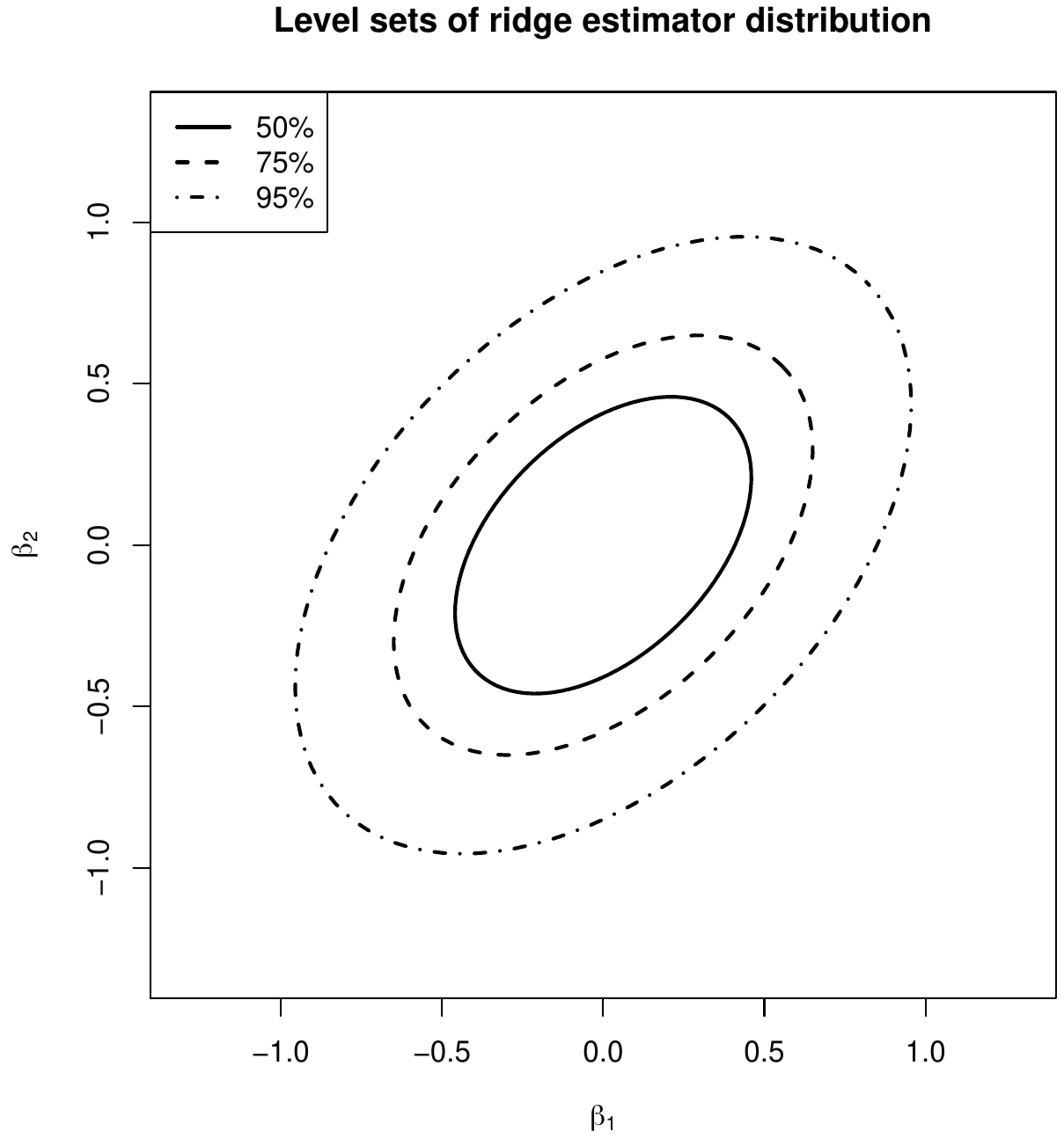
Level sets of the distribution of the ML (left panel) and ridge (right panel) regression estimators.

Example (Variance comparison)

Consider the design matrix:

[[math]] \begin{eqnarray*} \mathbf{X} & = & \left( \begin{array}{rr} -1 & 2 \\ 0 & 1 \\ 2 & -1 \\ 1 & 0 \end{array} \right). \end{eqnarray*} [[/math]]

The variances of the ML and ridge (with [math]\lambda=1[/math]) estimates of the regression coefficients then are:

[[math]] \begin{eqnarray*} \mbox{Var}(\hat{\bbeta}) & = & \sigma^2 \left( \begin{array}{rr} 0.3 & 0.2 \\ 0.2 & 0.3 \end{array} \right) \qquad \mbox{and} \qquad \mbox{Var}[\hat{\bbeta}(\lambda)] \, \, \, = \, \, \, \sigma^2 \left( \begin{array}{rr} 0.1524 & 0.0698 \\ 0.0698 & 0.1524 \end{array} \right). \end{eqnarray*} [[/math]]

These variances can be used to construct levels sets of the distribution of the estimates. The level sets that contain 50%, 75% and 95% of the distribution of the maximum likelihood and ridge regression estimates are plotted in Figure. In line with inequality \ref{form.VarInequalityMLandRidge} the level sets of the ridge regression estimate are smaller than that of the maximum likelihood one. The former thus varies less.

Example (Orthonormal design matrix, continued)

Assume the design matrix [math]\mathbf{X}[/math] is orthonormal. Then, [math]\mbox{Var} ( \hat{\bbeta} ) = \sigma^2 \mathbf{I}_{pp}[/math] and

[[math]] \begin{eqnarray*} \mbox{Var}[ \hat{\bbeta}(\lambda) ] & = & \sigma^2 \mathbf{W}_{\lambda} (\mathbf{X}^{\top} \mathbf{X})^{-1} \mathbf{W}_{\lambda}^{\top} \, \, \, = \, \, \, \sigma^2 (\mathbf{I}_{pp} + \lambda \mathbf{I}_{pp} )^{-1} \mathbf{I}_{pp} [ (\mathbf{I}_{pp} + \lambda \mathbf{I}_{pp} )^{-1} ]^{\top}\, \, \, = \, \, \, \sigma^2 (1 + \lambda )^{-2} \mathbf{I}_{pp}. \end{eqnarray*} [[/math]]

As the penalty parameter [math]\lambda[/math] is non-negative the former exceeds the latter. In particular, the expression after the utmost right equality sign vanishes as [math]\lambda \rightarrow \infty[/math].

Given [math]\lambda[/math] and [math]\mathbf{X}[/math], the random behavior of the estimator is thus known. In particular, when [math]n \lt p[/math], the variance is semi-positive definite and this [math]p[/math]-variate normal distribution is degenerate, i.e. there is no probability mass outside [math]\mathcal{R}(\mathbf{X})[/math] the subspace of [math]\mathbb{R}^p[/math] spanned by the rows of the [math]\mathbf{X}[/math].

Mean squared error

Previously, we motivated the ridge estimator as an ad hoc solution to collinearity. An alternative motivation comes from studying the Mean Squared Error (MSE) of the ridge regression estimator: for a suitable choice of [math]\lambda[/math] the ridge regression estimator may outperform the ML regression estimator in terms of the MSE. Before we prove this, we first derive the MSE of the ridge estimator and quote some auxiliary results. Note that, as the ridge regression estimator is compared to its ML counterpart, throughout this subsection [math]n \gt p[/math] is assumed to warrant the uniqueness of the latter.

Recall that (in general) for any estimator of a parameter [math]\theta[/math]:

[[math]] \begin{eqnarray*} \mbox{MSE}( \hat{\theta} ) & = & \mathbb{E} [ ( \hat{\theta} - \theta)^2 ] \, \, \, = \, \, \, \mbox{Var}( \hat{ \theta} ) + [\mbox{Bias} ( \hat{\theta} )]^2. \end{eqnarray*} [[/math]]

Hence, the MSE is a measure of the quality of the estimator. The MSE of the ridge regression estimator is:

[[math]] \begin{eqnarray} \mbox{MSE}[\hat{\bbeta}(\lambda)] & = & \mathbb{E} [ (\mathbf{W}_{\lambda} \, \hat{\bbeta} - \bbeta)^{\top} \, (\mathbf{W}_{\lambda} \, \hat{\bbeta} - \bbeta) ] \nonumber \\ & = & \mathbb{E} ( \hat{\bbeta}^{\top} \mathbf{W}_{\lambda}^{\top} \,\mathbf{W}_{\lambda} \, \hat{\bbeta} ) - \mathbb{E} ( \bbeta^{\top} \, \mathbf{W}_{\lambda} \, \hat{\bbeta}) - \mathbb{E} ( \hat{\bbeta}^{\top} \mathbf{W}_{\lambda}^{\top} \, \bbeta) + \mathbb{E} ( \bbeta^{\top} \bbeta) \nonumber \\ & = & \mathbb{E} ( \hat{\bbeta}^{\top} \mathbf{W}_{\lambda}^{\top} \,\mathbf{W}_{\lambda} \, \hat{\bbeta} ) - \mathbb{E} ( \bbeta^{\top} \, \mathbf{W}_{\lambda}^{\top} \mathbf{W}_{\lambda} \, \hat{\bbeta}) - \mathbb{E} ( \hat{\bbeta}^{\top} \mathbf{W}_{\lambda}^{\top} \, \mathbf{W}_{\lambda} \bbeta) + \mathbb{E} ( \bbeta^{\top} \mathbf{W}_{\lambda}^{\top} \,\mathbf{W}_{\lambda} \, \bbeta ) \nonumber \\ & & - \mathbb{E} ( \bbeta^{\top} \mathbf{W}_{\lambda}^{\top} \,\mathbf{W}_{\lambda} \, \bbeta ) + \mathbb{E} ( \bbeta^{\top} \, \mathbf{W}_{\lambda}^{\top} \mathbf{W}_{\lambda} \, \hat{\bbeta}) + \mathbb{E} ( \hat{\bbeta}^{\top} \mathbf{W}_{\lambda}^{\top} \, \mathbf{W}_{\lambda} \bbeta) \nonumber \\ & & - \mathbb{E} ( \bbeta^{\top} \, \mathbf{W}_{\lambda} \, \hat{\bbeta}) - \mathbb{E} ( \hat{\bbeta}^{\top} \mathbf{W}_{\lambda}^{\top} \, \bbeta) + \mathbb{E} ( \bbeta^{\top} \bbeta) \nonumber \\ & = & \mathbb{E} [ ( \hat{\bbeta} - \bbeta )^{\top} \mathbf{W}_{\lambda}^{\top} \, \mathbf{W}_{\lambda} \, (\hat{\bbeta} - \bbeta) ] \nonumber \\ & & - \bbeta^{\top} \mathbf{W}_{\lambda}^{\top} \,\mathbf{W}_{\lambda} \, \bbeta + \bbeta^{\top} \, \mathbf{W}_{\lambda}^{\top} \mathbf{W}_{\lambda} \, \bbeta + \bbeta^{\top} \mathbf{W}_{\lambda}^{\top} \, \mathbf{W}_{\lambda} \bbeta \nonumber \\ & & - \bbeta^{\top} \, \mathbf{W}_{\lambda} \, \bbeta - \bbeta^{\top} \mathbf{W}_{\lambda}^{\top} \, \bbeta + \bbeta^{\top} \bbeta \nonumber \\ & = & \mathbb{E} [ ( \hat{\bbeta} - \bbeta )^{\top} \mathbf{W}_{\lambda}^{\top} \, \mathbf{W}_{\lambda} \, (\hat{\bbeta} - \bbeta) ] + \bbeta^{\top} (\mathbf{W}_{\lambda} - \mathbf{I}_{pp})^{\top} (\mathbf{W}_{\lambda} - \mathbf{I}_{pp}) \bbeta \nonumber \\ & = & \sigma^2 \, \mbox{tr} [ \mathbf{W}_{\lambda} \, (\mathbf{X}^{\top} \mathbf{X})^{-1} \, \mathbf{W}_{\lambda}^{\top} ] + \bbeta^{\top} (\mathbf{W}_{\lambda} - \mathbf{I}_{pp})^{\top} (\mathbf{W}_{\lambda} - \mathbf{I}_{pp}) \bbeta. \label{form.ridgeMSE} \end{eqnarray} [[/math]]

In the last step we have used [math]\hat{\bbeta} \sim \mathcal{N}[ \bbeta, \sigma^2 \, (\mathbf{X}^{\top} \mathbf{X})^{-1} ][/math] and the expectation of the quadratic form of a multivariate random variable [math]\vvarepsilon \sim \mathcal{N}(\mmu_{\varepsilon}, \SSigma_{\varepsilon})[/math] that for a nonrandom symmetric positive definite matrix [math]\LLambda[/math] is (cf. ):

[[math]] \begin{eqnarray*} \mathbb{E} ( \vvarepsilon^{\top} \LLambda \, \vvarepsilon) & = & \mbox{tr} ( \LLambda \SSigma_{\varepsilon}) + \mmu_{\varepsilon}^{\top} \LLambda \mmu_{\varepsilon}, \end{eqnarray*} [[/math]]

of course replacing [math]\vvarepsilon[/math] by [math]\hat{\bbeta}[/math] in this expectation. The first summand in the final derived expression for [math]\mbox{MSE}[\hat{\bbeta}(\lambda)][/math] is the sum of the variances of the ridge estimator, while the second summand can be thought of the “squared bias” of the ridge estimator. In particular, [math]\lim_{\lambda \rightarrow \infty} \mbox{MSE}[\hat{\bbeta}(\lambda)] = \bbeta^{\top} \bbeta[/math], which is the squared biased for an estimator that equals zero (as does the ridge regression estimator in the limit).

Example Orthonormal design matrix

Assume the design matrix [math]\mathbf{X}[/math] is orthonormal. Then, [math]\mbox{MSE}[ \hat{\bbeta} ] = p \, \sigma^2[/math] and

[[math]] \begin{eqnarray*} \mbox{MSE}[ \hat{\bbeta}(\lambda) ] & = & p \, \sigma^2 (1+ \lambda)^{-2} + \lambda^2 (1+ \lambda)^{-2} \bbeta^{\top} \bbeta. \end{eqnarray*} [[/math]]

The latter achieves its minimum at: [math]\lambda = p \sigma^2 / \bbeta^{\top} \bbeta[/math].

For some [math]\lambda[/math] the ridge regression estimator yields a lower MSE than the ML regression estimator:

Theorem 2 of

There exists [math]\lambda \gt 0[/math] such that [math]\mbox{MSE}[\hat{\bbeta}(\lambda)] \lt \mbox{MSE}[\hat{\bbeta}(0)] = \mbox{MSE}(\hat{\bbeta})[/math].

Show Proof

See theorem.■

This result of is generalized by to the class of design matrices [math]\mathbf{X}[/math] with [math]\mbox{rank}(\mathbf{X}) \lt p[/math].

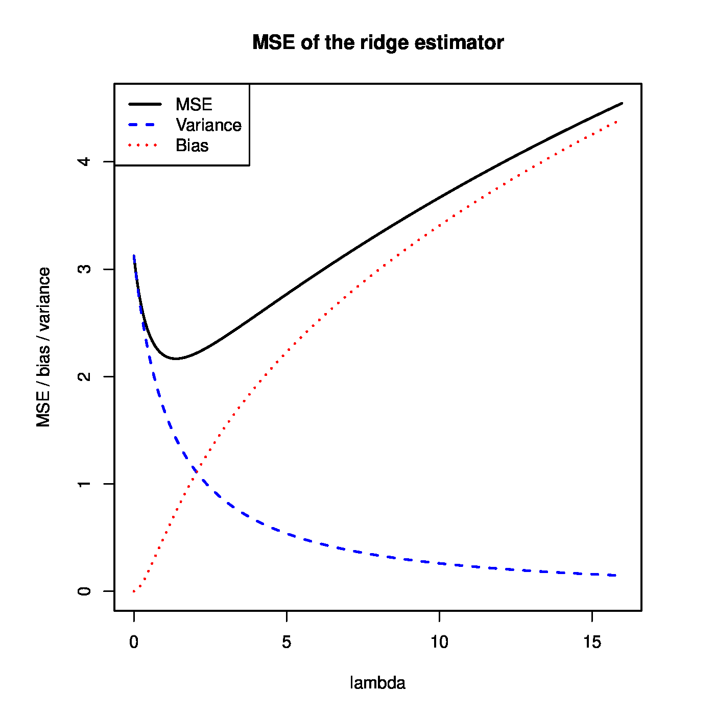
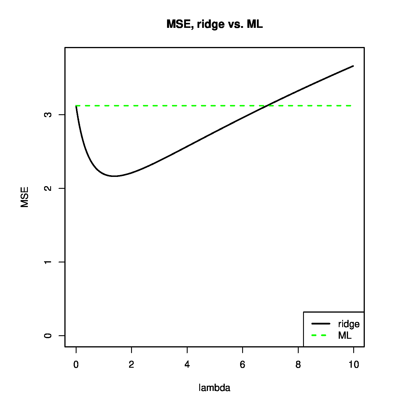
Theorem can be used to illustrate that the ridge regression estimator strikes a balance between the bias and variance. This is illustrated in the left panel of Figure. For small [math]\lambda[/math], the variance of the ridge estimator dominates the MSE. This may be understood when realizing that in this domain of [math]\lambda[/math] the ridge estimator is close to the unbiased ML regression estimator. For large [math]\lambda[/math], the variance vanishes and the bias dominates the MSE. For small enough values of [math]\lambda[/math], the decrease in variance of the ridge regression estimator exceeds the increase in its bias. As the MSE is the sum of these two, the MSE first decreases as [math]\lambda[/math] moves away from zero. In particular, as [math]\lambda = 0[/math] corresponds to the ML regression estimator, the ridge regression estimator yields a lower MSE for these values of [math]\lambda[/math]. In the right panel of Figure [math]\mbox{MSE}[ \hat{\bbeta}(\lambda)] \lt \mbox{MSE}[ \hat{\bbeta}(0)][/math] for [math]\lambda \lt 7[/math] (roughly) and the ridge estimator outperforms the ML estimator.

Left panel: mean squared error, and its ‘bias’ and ‘variance’ parts, of the ridge regression estimator (for artificial data). Right panel: mean squared error of the ridge and ML estimator of the regression coefficient vector (for the same artificial data).

Besides another motivation behind the ridge regression estimator, the use of Theorem is limited. The optimal choice of [math]\lambda[/math] depends on the quantities [math]\bbeta[/math] and [math]\sigma^2[/math]. These are unknown in practice. Then, the penalty parameter is chosen in a data-driven fashion (see e.g. Section Cross-validation and various other places).

Theorem may be of limited practical use, it does give insight in when the ridge regression estimator may be preferred over its ML counterpart. Ideally, the range of penalty parameters for which the ridge regression estimator outperforms -- in the MSE sense -- the ML regression estimator is as large as possible. The factors that influence the size of this range may be deduced from the optimal penalty [math]\lambda_{\mbox{{\tiny opt}}} = \sigma^2 (\bbeta^{\top} \bbeta / p)^{-1}[/math] found under the assumption of an orthonormal [math]\mathbf{X}[/math] (see Example). But also from the bound on the penalty parameter, [math]\lambda_{\mbox{{\tiny max}}} = 2 \sigma^2 (\bbeta^{\top} \bbeta )^{-1}[/math] such that [math]MSE[\hat{\bbeta}(\lambda)] \lt MSE[\hat{\bbeta}(0)][/math] for all [math]\lambda \in (0, \lambda_{\mbox{{\tiny max}}})[/math], derived in the proof of Theorem. Firstly, an increase of the error variance [math]\sigma^2[/math] yields a larger [math]\lambda_{\mbox{{\tiny opt}}}[/math] and [math]\lambda_{\mbox{{\tiny max}}}[/math]. Put differently, more noisy data benefits the ridge regression estimator. Secondly, [math]\lambda_{\mbox{{\tiny opt}}}[/math] and [math]\lambda_{\mbox{{\tiny max}}}[/math] also become larger when their denominators decreases. The denominator [math]\bbeta^{\top} \bbeta / p[/math] may be viewed as an estimator of the ‘signal’ variance ‘[math]\sigma^2_{\beta}[/math]’. A quick conclusion would be that ridge regression profits from less signal. But more can be learned from the denominator. Contrast the two regression parameters [math]\bbeta_{\mbox{{\tiny unif}}} = \mathbf{1}_p[/math] and [math]\bbeta_{\mbox{{\tiny sparse}}}[/math] which comprises of only zeros except the first element which equals [math]p[/math], i.e. [math]\bbeta_{\mbox{{\tiny sparse}}} = (p, 0, \ldots, 0)^{\top}[/math]. Then, the [math]\bbeta_{\mbox{{\tiny unif}}}[/math] and [math]\bbeta_{\mbox{{\tiny sparse}}}[/math] have comparable signal in the sense that [math]\sum_{j=1}^p \beta_j = p[/math]. The denominator of [math]\lambda_{\mbox{{\tiny opt}}}[/math] corresponding both parameters equals [math]1[/math] and [math]p[/math], respectively. This suggests that ridge regression will perform better in the former case where the regression parameter is not dominated by a few elements but rather all contribute comparably to the explanation of the variation in the response. Of course, more factors contribute. For instance, collinearity among the columns of [math]\mathbf{X}[/math], which gave rise to ridge regression in the first place.

Theorem can also be used to conclude on the biasedness of the ridge regression estimator. The Gauss-Markov theorem states (under some assumptions) that the ML regression estimator is the best linear unbiased estimator (BLUE) with the smallest MSE. As the ridge regression estimator is a linear estimator and outperforms (in terms of MSE) this ML estimator, it must be biased (for it would otherwise refute the Gauss-Markov theorem).

Constrained estimation

The ad-hoc fix of to super-collinearity of the design matrix (and, consequently the singularity of the matrix [math]\mathbf{X}^{\top} \mathbf{X}[/math]) has been motivated post-hoc. The ridge regression estimator minimizes the ridge loss function, which is defined as:

[[math]] \begin{eqnarray} \mathcal{L}_{\mbox{{\tiny ridge}}}(\bbeta; \lambda) & = & \| \mathbf{Y} - \mathbf{X} \bbeta \|^2_2 + \lambda \| \bbeta \|^2_2 \, \, \, = \, \, \, \sum\nolimits_{i=1}^n (Y_i - \mathbf{X}_{i\ast} \bbeta)^2 + \lambda \sum\nolimits_{j=1}^p \beta_j^2. \label{form.ridgeLossFunction} \end{eqnarray} [[/math]]

This loss function is the traditional sum-of-squares augmented with a penalty. The particular form of the penalty, [math]\lambda \| \bbeta \|^2_2[/math] is referred to as the ridge penalty and [math]\lambda[/math] as the penalty parameter. For [math]\lambda=0[/math], minimization of the ridge loss function yields the ML estimator (if it exists). For any [math]\lambda \gt 0[/math], the ridge penalty contributes to the loss function, affecting its minimum and its location. The minimum of the sum-of-squares is well-known. The minimum of the ridge penalty is attained at [math]\bbeta = \mathbf{0}_{p}[/math] whenever [math]\lambda \gt 0[/math]. The [math]\bbeta[/math] that minimizes [math]\mathcal{L}_{\mbox{{\tiny ridge}}}(\bbeta; \lambda)[/math] then balances the sum-of-squares and the penalty. The effect of the penalty in this balancing act is to shrink the regression coefficients towards zero, its minimum. In particular, the larger [math]\lambda[/math], the larger the contribution of the penalty to the loss function, the stronger the tendency to shrink non-zero regression coefficients to zero (and decrease the contribution of the penalty to the loss function). This motivates the name ‘penalty’ as non-zero elements of [math]\bbeta[/math] increase (or penalize) the loss function.

To verify that the ridge regression estimator indeed minimizes the ridge loss function, proceed as usual. Take the derivative with respect to [math]\bbeta[/math]:

[[math]] \begin{eqnarray*} \frac{\partial}{\partial \bbeta} \mathcal{L}_{\mbox{{\tiny ridge}}}(\bbeta; \lambda) & = & -2 \mathbf{X}^{\top} (\mathbf{Y} - \mathbf{X} \bbeta) + 2 \lambda \mathbf{I}_{pp} \bbeta \, \, \, = \, \, \, -2 \mathbf{X}^{\top} \mathbf{Y} + 2 ( \mathbf{X}^{\top} \mathbf{X} + \lambda \mathbf{I}_{pp}) \bbeta. \end{eqnarray*} [[/math]]

Equate the derivative to zero and solve for [math]\bbeta[/math]. This yields the ridge regression estimator.

The ridge estimator is thus a stationary point of the ridge loss function. A stationary point corresponds to a minimum if the Hessian matrix with second order partial derivatives is positive definite. The Hessian of the ridge loss function is

[[math]] \begin{eqnarray*} \frac{\partial^2}{\partial \bbeta \, \partial \bbeta^{\top}} \mathcal{L}_{\mbox{{\tiny ridge}}}(\bbeta; \lambda) & = & 2 ( \mathbf{X}^{\top} \mathbf{X} + \lambda \mathbf{I}_{pp}). \end{eqnarray*} [[/math]]

This Hessian is the sum of the (semi-)positive definite matrix [math]\mathbf{X}^{\top} \mathbf{X}[/math] and the positive definite matrix [math]\lambda \, \mathbf{I}_{pp}[/math]. Lemma 14.2.4 of then states that the sum of these matrices is itself a positive definite matrix. Hence, the Hessian is positive definite and the ridge loss function has a stationary point at the ridge estimator, which is a minimum.

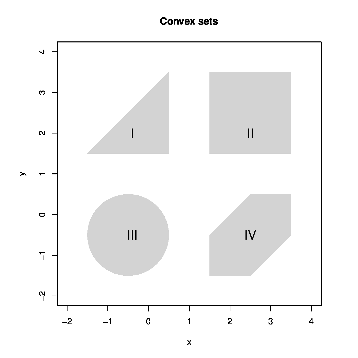
The ridge regression estimator minimizes the ridge loss function. It rests to verify that it is a global minimum. To this end we introduce the concept of a convex function. As a prerequisite, a set [math]\mathcal{S} \subset \mathbb{R}^p[/math] is called convex if for all [math]\bbeta_1, \bbeta_2 \in \mathcal{S}[/math] their weighted average [math]\bbeta_{\theta} = (1 - \theta) \bbeta_1 + \theta \bbeta_2[/math] for all [math]\theta \in [0, 1][/math] is itself an element of [math]\mathcal{S}[/math], thus [math]\bbeta_{\theta} \in \mathcal{S}[/math]. If for all [math]\theta \in (0, 1)[/math], the weighted average [math]\bbeta_{\theta}[/math] is inside [math]\mathcal{S}[/math] and not on its boundary, the set is called strictly convex. Examples of (strictly) convex and nonconvex sets are depicted in Figure. A function [math]f(\cdot)[/math] is (strictly) convex if the set [math]\{ y \, : \, y \geq f(\bbeta) \mbox{ for all } \bbeta \in \mathcal{S} \mbox{ for any convex } \mathcal{S} \}[/math], called the epigraph of [math]f(\cdot)[/math], is (strictly) convex. Examples of (strictly) convex and nonconvex functions are depicted in Figure. The ridge loss function is the sum of two parabola's: one is at least convex and the other strictly convex in [math]\bbeta[/math]. The sum of a convex and strictly convex function is itself strictly convex (see Lemma 9.4.2 of ). The ridge loss function is thus strictly convex. Theorem 9.4.1 of then warrants, by the strict convexity of the ridge loss function, that the ridge regression estimator is a global minimum.

From the ridge loss function the limiting behavior of the variance of the ridge regression estimator can be understood. The ridge penalty with its minimum [math]\bbeta = \mathbf{0}_{p}[/math] does not involve data and, consequently, the variance of its minimum equals zero. With the ridge regression estimator being a compromise between the maximum likelihood estimator and the minimum of the penalty, so is its variance a compromise of their variances. As [math]\lambda[/math] tends to infinity, the ridge regression estimator and its variance converge to the minimizer of the loss function and the variance of the minimizer, respectively. Hence, in the limit (large [math]\lambda[/math]) the variance of the ridge regression estimator vanishes. Understandably, as the penalty now fully dominates the loss function and, consequently, it does no longer involve data (i.e. randomness).

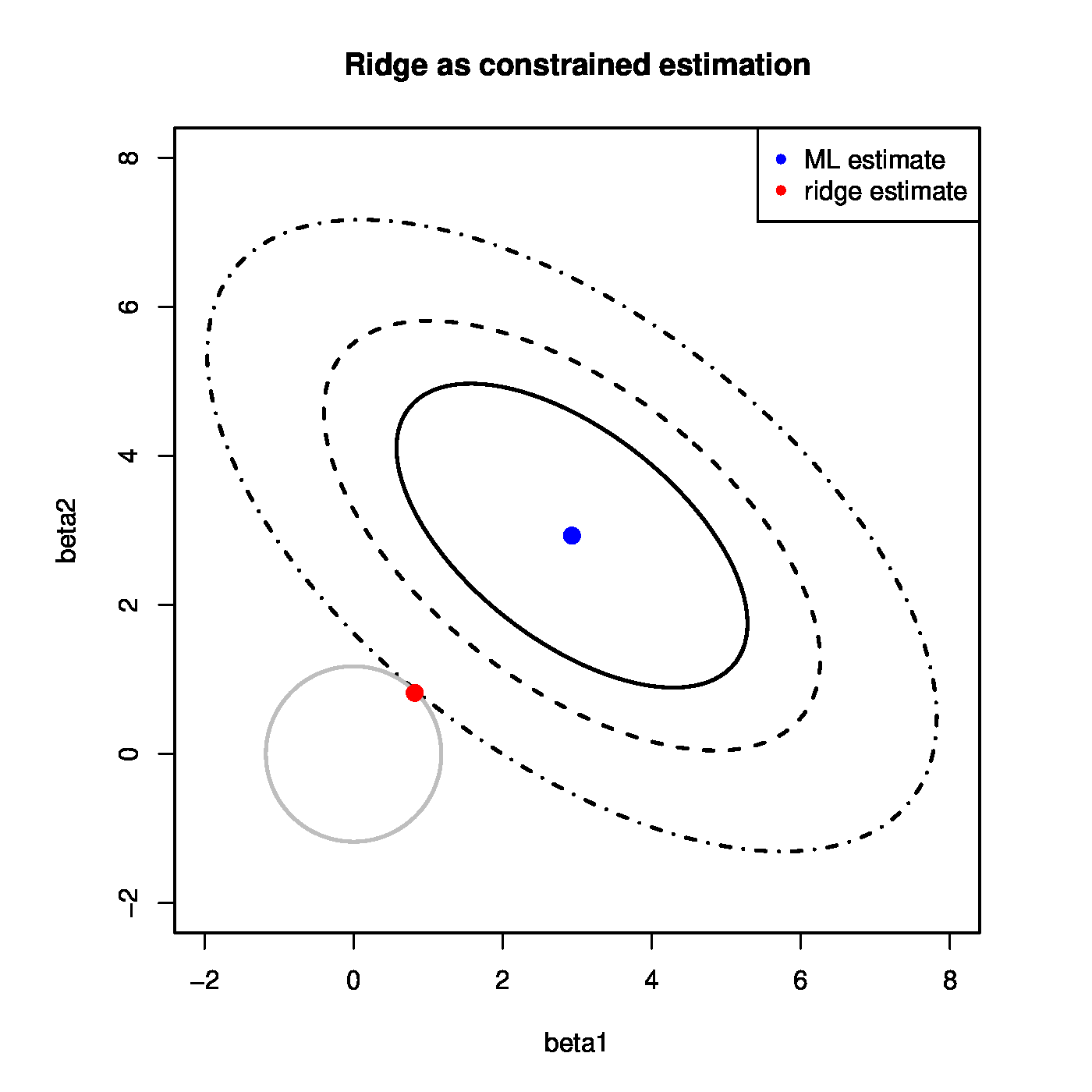
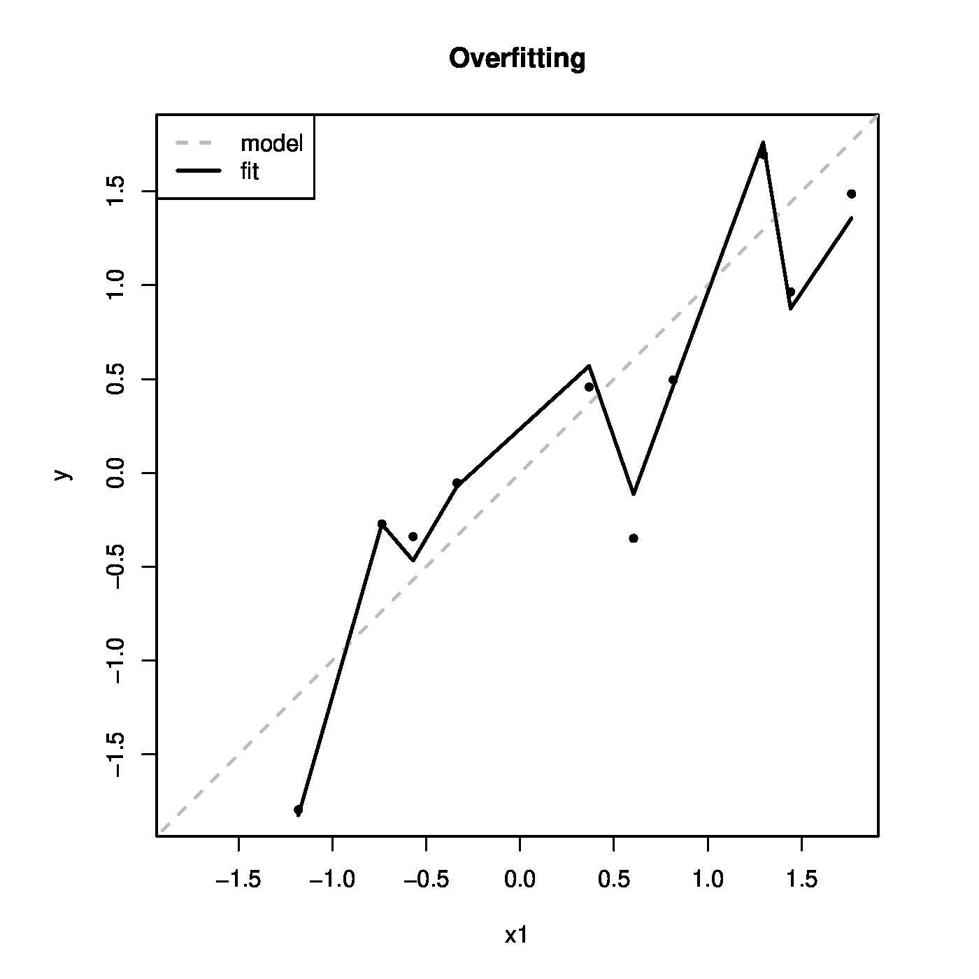
Figure: Top panels show examples of convex (left) and nonconvex (right) sets. Middle panels show examples of convex (left) and nonconvex (right) functions. The left bottom panel illustrates the ridge estimation as a constrained estimation problem. The ellipses represent the contours of the ML loss function, with the blue dot at the center the ML estimate. The circle is the ridge parameter constraint. The red dot is the ridge estimate. It is at the intersection of the ridge constraint and the smallest contour with a non-empty intersection with the constraint. The right bottom panel shows the data corresponding to Example. The grey line represents the ‘true’ relationship, while the black line the fitted one.

Above it has been shown that the ridge estimator can be defined as:

[[math]] \begin{eqnarray} \label{form.ridgeEstViaPenEst} \hat{\bbeta}(\lambda) & = & \arg \min_{\bbeta} \| \mathbf{Y} - \mathbf{X} \, \bbeta \|^2_2 + \lambda \| \bbeta \|^2_2. \end{eqnarray} [[/math]]

This minimization problem can be reformulated into the following constrained optimization problem:

[[math]] \begin{eqnarray} \label{form.constrEstProblemRidge} \hat{\bbeta}(\lambda) & = & \arg \min_{\| \bbeta \|_2^2 \leq c} \| \mathbf{Y} - \mathbf{X} \, \bbeta \|^2_2, \end{eqnarray} [[/math]]

for some suitable [math]c \gt 0[/math]. The constrained optimization problem (\ref{form.constrEstProblemRidge}) can be solved by means of the Karush-Kuhn-Tucker (KKT) multiplier method, which minimizes a function subject to inequality constraints.

The constrained estimation interpretation of the ridge regression estimator is illustrated in the left bottom panel of Figure. It shows the level sets of the sum-of-squares criterion and centered around zero the circular ridge parameter constraint, parametrized by [math]\{ \bbeta \, : \, \| \bbeta \|_2^2 = \beta_1^2 + \beta_2^2 \leq c \}[/math] for some [math]c \gt 0[/math]. The ridge regression estimator is then the point where the sum-of-squares' smallest level set hits the constraint. Exactly at that point the sum-of-squares is minimized over those [math]\bbeta[/math]'s that live on or inside the constraint. In the high-dimensional setting the ellipsoidal level sets are degenerated. For instance, the 2-dimensional case of the left bottom panel of Figure the ellipsoids would then be lines, but the geometric interpretation is unaltered.

The ridge regression estimator is always to be found on the boundary of the ridge parameter constraint and is never an interior point. To see this assume, for simplicity, that the [math]\mathbf{X}^{\top} \mathbf{X}[/math] matrix is of full rank. The radius of the ridge parameter constraint can then be bounded as follows:

[[math]] \begin{eqnarray*} \| \hat{\bbeta} ( \lambda) \|_2^2 & = & \mathbf{Y}^{\top} \mathbf{X} (\mathbf{X}^{\top} \mathbf{X} + \lambda \mathbf{I}_{pp})^{-2} \mathbf{X}^{\top} \mathbf{Y} \, \, \,\leq \, \, \, \mathbf{Y}^{\top} \mathbf{X} (\mathbf{X}^{\top} \mathbf{X})^{-2} \mathbf{X}^{\top} \mathbf{Y} \, \, \, = \, \, \, \| \hat{\bbeta}^{\mbox{{\tiny ml}}} \|_2^2. \end{eqnarray*} [[/math]]

The inequality in the display above follows from

1. [math]\mathbf{X}^{\top} \mathbf{X} \succ 0[/math] and [math]\lambda \mathbf{I}_{pp} \succ 0[/math],
2. [math]\mathbf{X}^{\top} \mathbf{X} + \lambda \mathbf{I}_{pp} \succ \mathbf{X}^{\top} \mathbf{X}[/math] (due to Lemma 14.2.4 of ),
3. and [math](\mathbf{X}^{\top} \mathbf{X})^{-2} \succ (\mathbf{X}^{\top} \mathbf{X} + \lambda \mathbf{I}_{pp})^{-2}[/math] (inferring Corollary 7.7.4 of ).

The ridge regression estimator is thus always on the boundary or in a circular constraint centered around the origin with a radius that is smaller than the size of the maximum likelihood estimator. Moreover, the constrained estimation formulation of the ridge regression estimator then implies that the latter must be on the boundary of the constraint.

The relevance of viewing the ridge regression estimator as the solution to a constrained estimation problem becomes obvious when considering a typical threat to high-dimensional data analysis: overfitting. Overfitting refers to the phenomenon of modelling the noise rather than the signal. In case the true model is parsimonious (few covariates driving the response) and data on many covariates are available, it is likely that a linear combination of all covariates yields a higher likelihood than a combination of the few that are actually related to the response. As only the few covariates related to the response contain the signal, the model involving all covariates then cannot but explain more than the signal alone: it also models the error. Hence, it overfits the data. In high-dimensional settings overfitting is a real threat. The number of explanatory variables exceeds the number of observations. It is thus possible to form a linear combination of the covariates that perfectly explains the response, including the noise.

Large estimates of regression coefficients are often an indication of overfitting. Augmentation of the estimation procedure with a constraint on the regression coefficients is a simple remedy to large parameter estimates. As a consequence it decreases the probability of overfitting. Overfitting is illustrated in the next example.

Example (Overfitting)

Consider an artificial data set comprising of ten observations on a response [math]Y_i[/math] and nine covariates [math]X_{i,j}[/math]. All covariate data are sampled from the standard normal distribution: [math]X_{i,j} \sim \mathcal{N}(0, 1)[/math]. The response is generated by [math]Y_i = X_{i,1} + \varepsilon_i[/math] with [math]\varepsilon_{i} \sim \mathcal{N}(0, \tfrac{1}{4})[/math]. Hence, only the first covariate contributes to the response.

The regression model [math]Y_i = \sum_{j=1}^9 X_{i,j} \beta_j+ \varepsilon_i[/math] is fitted to the artificial data using R. This yields the regression parameter estimates:

[[math]] \begin{eqnarray*} \hat{\bbeta}^{\top} & = & (0.048, -2.386, -5.528, 6.243, -4.819, 0.760, -3.345, -4.748, 2.136). \end{eqnarray*} [[/math]]

As [math]\bbeta^{\top} = (1, 0, \ldots, 0)[/math], many regression coefficient are clearly over-estimated.

The fitted values [math]\widehat{Y}_i = \mathbf{X}_i \hat{\bbeta}[/math] are plotted against the values of the first covariates in the right bottom panel of Figure. As a reference the line [math]x=y[/math] is added, which represents the ‘true’ model. The fitted model follows the ‘true’ relationship. But it also captures the deviations from this line that represent the errors.

Penalty parameter selection

Throughout the introduction of the ridge regression estimator and the subsequent discussion of its properties, we considered the penalty parameter known or ‘given’. In practice, it is unknown and the user needs to make an informed decision on its value. We present several strategies to facilitate such a decision. Prior to that, we discuss some sanity requirements one may wish to impose on the ridge regression estimator. Those requirements do not yield a specific choice of the penalty parameter but they specify a domain of sensible penalty parameter values.

Degrees of freedom

The degrees of freedom consumed by ridge regression is calculated. The degrees of freedom may be used in combination with an information criterion to decide on the value of the penalty parameter. Recall from ordinary regression that: [math]\widehat{\mathbf{Y}} = \mathbf{X} (\mathbf{X}^{\top} \mathbf{X})^{-1} \mathbf{X}^{\top} \mathbf{Y} = \mathbf{H} \mathbf{Y}[/math] where [math]\mathbf{H}[/math] is the hat matrix. The degrees of freedom used in the regression is then equal to [math]\mbox{tr}(\mathbf{H})[/math], the trace of [math]\mathbf{H}[/math]. In particular, if [math] \mathbf{X}[/math] is of full rank, i.e. [math]\mbox{rank}(\mathbf{X}) = p[/math], then [math]\mbox{tr}(\mathbf{H}) = p[/math].

By analogy, the ridge-version of the hat matrix is defined as [math]\mathbf{H}(\lambda) := \mathbf{X} (\mathbf{X}^{\top} \mathbf{X} + \lambda \mathbf{I}_{pp})^{-1} \mathbf{X}^{\top}[/math]. Continuing this analogy, the degrees of freedom of ridge regression is given by the trace of the ridge hat matrix [math]\mathbf{H}(\lambda)[/math]:

[[math]] \begin{eqnarray*} \mbox{tr}[ \mathbf{H}(\lambda)] & = & \mbox{tr}[ \mathbf{X} (\mathbf{X}^{\top} \mathbf{X} + \lambda \mathbf{I}_{pp})^{-1} \mathbf{X}^{\top} ] \, \, \, = \, \, \, \sum\nolimits_{j=1}^p (\mathbf{D}_x^{\top} \mathbf{D}_x)_{jj} [(\mathbf{D}_x^{\top} \mathbf{D}_x)_{jj} + \lambda]^{-1}. \end{eqnarray*} [[/math]]

The degrees of freedom consumed by ridge regression is monotone decreasing in [math]\lambda[/math]. In particular, [math]\lim_{\lambda \rightarrow \infty} \mbox{tr}[ \mathbf{H}(\lambda)] = 0[/math]. That is, in the limit no information from [math]\mathbf{X}[/math] is used. Indeed, [math]\bbeta[/math] is forced to equal [math]\mathbf{0}_{p}[/math] which is not derived from data.

Cross-validation

Instead of choosing the penalty parameter to balance model fit with model complexity, cross-validation requires it (i.e. the penalty parameter) to yield a model with good prediction performance. Commonly, this performance is evaluated on novel data. Novel data need not be easy to come by and one has to make do with the data at hand. The setting of ‘original’ and novel data is then mimicked by sample splitting: the data set is divided into two (groups of samples). One of these two data sets, called the training set, plays the role of ‘original’ data on which the model is built. The second of these data sets, called the test set, plays the role of the ‘novel’ data and is used to evaluate the prediction performance (often operationalized as the loglikelihood or the prediction error) of the model built on the training data set. This procedure (model building and prediction evaluation on training and test set, respectively) is done for a collection of possible penalty parameter choices. The penalty parameter that yields the model with the best prediction performance is to be preferred. The thus obtained performance evaluation depends on the actual split of the data set. To remove this dependence, the data set is split many times into a training and test set. Per split the model parameters are estimated for all choices of [math]\lambda[/math] using the training data and estimated parameters are evaluated on the corresponding test set. The penalty parameter, that on average over the test sets performs best (in some sense), is then selected.

When the repetitive splitting of the data set is done randomly, samples may accidently end up in a fast majority of the splits in either training or test set. Such samples may have an unbalanced influence on either model building or prediction evaluation. To avoid this [math]k[/math]-fold cross-validation structures the data splitting. The samples are divided into [math]k[/math] more or less equally sized exhaustive and mutually exclusive subsets. In turn (at each split) one of these subsets plays the role of the test set while the union of the remaining subsets constitutes the training set. Such a splitting warrants a balanced representation of each sample in both training and test set over the splits. Still the division into the [math]k[/math] subsets involves a degree of randomness. This may be fully excluded when choosing [math]k=n[/math]. This particular case is referred to as leave-one-out cross-validation (LOOCV). For illustration purposes the LOOCV procedure is detailed fully below:

LOOCV

0. Define a range of interest for the penalty parameter.
1. Divide the data set into training and test set comprising samples [math]\{1, \ldots, n\} \setminus i[/math] and [math]\{ i \}[/math], respectively.
2. Fit the linear regression model by means of ridge estimation for each [math]\lambda[/math] in the grid using the training set. This yields:
   [[math]] \begin{eqnarray*} \hat{\bbeta}_{-i}(\lambda) & = & ( \mathbf{X}_{-i, \ast}^{\top} \mathbf{X}_{-i, \ast} + \lambda \mathbf{I}_{pp})^{-1} \mathbf{X}_{-i, \ast}^{\top} \mathbf{Y}_{-i} \end{eqnarray*} [[/math]]
   and the corresponding estimate of the error variance [math]\hat{\sigma}_{-i}^2(\lambda)[/math].
3. Evaluate the prediction performance of these models on the test set by [math]\log\{L[Y_i, \mathbf{X}_{i, \ast}; \hat{\bbeta}_{-i}(\lambda), \hat{\sigma}_{-i}^2(\lambda)]\}[/math]. Or, by the prediction error [math]|Y_i - \mathbf{X}_{i, \ast} \hat{\bbeta}_{-i}(\lambda)|[/math], possibly squared.
4. Repeat steps 1) to 3) such that each sample plays the role of the test set once.
5. Average the prediction performances of the test sets at each grid point of the penalty parameter:
   [[math]] \begin{eqnarray*} n^{-1} \sum\nolimits_{i = 1}^n \log\{L[Y_i, \mathbf{X}_{i, \ast}; \hat{\bbeta}_{-i}(\lambda), \hat{\sigma}_{-i}^2(\lambda)]\}. \end{eqnarray*} [[/math]]
   The quantity above is called the cross-validated loglikelihood. It is an estimate of the prediction performance of the model corresponding to this value of the penalty parameter on novel data.
6. The value of the penalty parameter that maximizes the cross-validated loglikelihood is the value of choice.

The procedure is straightforwardly adopted to [math]k[/math]-fold cross-validation, a different criterion, and different estimators.

In the LOOCV procedure above resampling can be avoided when the predictive performance is measured by Allen's PRESS (Predicted Residual Error Sum of Squares) statistic . For then, the LOOCV predictive performance can be expressed analytically in terms of the known quantities derived from the design matrix and response (as pointed out but not detailed in ). Define the optimal penalty parameter to minimize Allen's PRESS statistic:

[[math]] \begin{eqnarray*} \lambda_{\mbox{{\tiny opt}}} = \arg \min_{\lambda} n^{-1} \sum\nolimits_{i=1}^n [Y_i - \mathbf{X}_{i, \ast} \hat{\bbeta}_{-i}(\lambda)]^2 \, \, \, = \, \, \, \arg \min_{\lambda} n^{-1} \| \mathbf{B}(\lambda) [\mathbf{I}_{nn} - \mathbf{H}(\lambda)] \mathbf{Y} \|_ F^2, \end{eqnarray*} [[/math]]

where [math]\mathbf{B}(\lambda)[/math] is diagonal with [math][\mathbf{B}(\lambda)]_{ii} = [ 1 - \mathbf{H}_{ii}(\lambda)]^{-1}[/math]. The second equality in the preceding display is elaborated in Exercise. Its main takeaway is that the predictive performance for a given [math]\lambda[/math] can be assessed directly from the ridge hat matrix and the response vector without the recalculation of the [math]n[/math] leave-one-out ridge regression estimators. Computationally, this is a considerable gain.

No such analytic expression of the cross-validated loss as above exists for general [math]K[/math]-fold cross-validation, but considerable computational gain can nonetheless be achieved . This exploits the fact that the ridge regression estimator appears in Allen's PRESS statistics -- and the likelihood -- only in combination with the design matrix, together forming the linear predictor. There is thus no need to evaluate the estimator itself when interest is only in its predictive performance. Then, if [math]\mathcal{G}_1, \ldots, \mathcal{G}_K \subset \{1, \ldots, n\}[/math] are the mutually exclusive and exhaustive [math]K[/math]-fold sample index sets, the linear predictor for the [math]k[/math]-th fold can be expressed as:

[[math]] \begin{eqnarray} \label{form.efficientCVlinearpredictor} \mathbf{X}_{\mathcal{G}_k, \ast} \hat{\bbeta}_{-\mathcal{G}_k}(\lambda) & = & \lambda^{-1} \mathbf{X}_{\mathcal{G}_k, \ast} \mathbf{X}_{-\mathcal{G}_k, \ast}^{\top} (\lambda^{-1} \mathbf{X}_{-\mathcal{G}_k, \ast} \mathbf{X}_{-\mathcal{G}_k, \ast}^{\top} + \mathbf{I}_{n-|\mathcal{G}_k|, n-|\mathcal{G}_k|})^{-1} \mathbf{Y}_{-\mathcal{G}_k, \ast}, \end{eqnarray} [[/math]]

where we have used the Woodbury identity again. Finally, for each fold the computationally most demanding matrices of this expression, [math]\mathbf{X}_{\mathcal{G}_k, \ast} \mathbf{X}_{-\mathcal{G}_k, \ast}^{\top}[/math] and [math]\mathbf{X}_{-\mathcal{G}_k, \ast} \mathbf{X}_{-\mathcal{G}_k, \ast}^{\top}[/math], are both submatrices of [math]\mathbf{X} \mathbf{X}^{\top}[/math]. If this matrix is evaluated prior to the cross-validation loop, all calculations inside the loop involve only matrices of dimensions [math]n \times n[/math], maximally.

General References

van Wieringen, Wessel N. (2021). "Lecture notes on ridge regression". arXiv:1509.09169 [stat.ME].

References

- 1.0 1.1 1.2 1.3 Harville, D. A. (2008).Matrix Algebra From a Statistician's Perspective.Springer, New York
- Ishwaran, H. and Rao, J. S. (2014).Geometry and properties of generalized ridge regression in high dimensions.Contempory Mathematics, 622, 81--93
- 3.0 3.1 3.2 3.3 Hoerl, A. E. and Kennard, R. W. (1970).Ridge regression: biased estimation for nonorthogonal problems.Technometrics, 12(1), 55--67
- Mathai, A. M. and Provost, S. B. (1992).Quadratic Forms in Random Variables: Theory and Applications.Dekker
- 5.0 5.1 Theobald, C. M. (1974).Generalizations of mean square error applied to ridge regression.Journal of the Royal Statistical Society. Series B (Methodological), 36(1), 103--106
- Farebrother, R. W. (1976).Further results on the mean square error of ridge regression.Journal of the Royal Statistical Society, Series B (Methodological), pages 248--250
- Rao, C. R. (1973).Linear Statistical Inference and its Applications.John Wiley & Sons
- 8.0 8.1 Fletcher, R. (2008).Practical Methods of Optimization, 2nd Edition.John Wiley, New York
- Horn, R. A. and Johnson, C. R. (2012).Matrix analysis.Cambridge University Press
- Allen, D. M. (1974).The relationship between variable selection and data agumentation and a method for prediction.Technometrics, 16(1), 125--127
- Golub, G. H., Heath, M., and Wahba, G. (1979).Generalized cross-validation as a method for choosing a good ridge parameter.Technometrics, 21(2), 215--223
- van de Wiel, M. A., van Nee, M. M., and Rauschenberger, A. (2021).Fast cross-validation for multi-penalty ridge regression.Journal of Computational and Graphical Statistics, (just-accepted), 1--31