Estimation, moments, and the bayesian connection

[math] \require{textmacros} \def \bbeta {\bf \beta} \def\fat#1{\mbox{\boldmath$#1$}} \def\reminder#1{\marginpar{\rule[0pt]{1mm}{11pt}}\textbf{#1}} \def\SSigma{\bf \Sigma} \def\ttheta{\bf \theta} \def\aalpha{\bf \alpha} \def\bbeta{\bf \beta} \def\ddelta{\bf \delta} \def\eeta{\bf \eta} \def\llambda{\bf \lambda} \def\ggamma{\bf \gamma} \def\nnu{\bf \nu} \def\vvarepsilon{\bf \varepsilon} \def\mmu{\bf \mu} \def\nnu{\bf \nu} \def\ttau{\bf \tau} \def\SSigma{\bf \Sigma} \def\TTheta{\bf \Theta} \def\XXi{\bf \Xi} \def\PPi{\bf \Pi} \def\GGamma{\bf \Gamma} \def\DDelta{\bf \Delta} \def\ssigma{\bf \sigma} \def\UUpsilon{\bf \Upsilon} \def\PPsi{\bf \Psi} \def\PPhi{\bf \Phi} \def\LLambda{\bf \Lambda} \def\OOmega{\bf \Omega} [/math]

Estimation

In the absence of an analytic expression for the optimum of the lasso loss function, much attention is devoted to numerical procedures to find it.

Quadratic programming

In the original lasso paper reformulates the lasso optimization problem to a quadratic program. A quadratic problem optimizes a quadratic form subject to linear constraints. This is a well-studied optimization problem for which many readily available implementations exist (e.g., the quadprog-package in R). The quadratic program that is equivalent to the lasso regression problem, which minimizes the least squares criterion, [math]\| \mathbf{Y} - \mathbf{X} \bbeta \|_2^2[/math] subject to [math]\| \bbeta \|_1 \lt c(\lambda_1)[/math], is:

[[math]] \begin{eqnarray} \label{form:quadProgam} \min_{\mathbf{R} \bbeta \geq \mathbf{0}} \tfrac{1}{2} (\mathbf{Y} - \mathbf{X} \bbeta )^{\top} (\mathbf{Y} - \mathbf{X} \bbeta ), \end{eqnarray} [[/math]]

where [math]\mathbf{R}[/math] is a [math]q \times p[/math] dimensional linear constraint matrix that specifies the linear constraints on the parameter [math]\bbeta[/math]. For [math]p=2[/math] the domain implied by lasso parameter constraint [math]\{ \bbeta \in \mathbb{R}^2 : \| \bbeta \|_1 \lt c(\lambda_1) \}[/math] is equal to:

[[math]] \begin{eqnarray*} & & \{ \bbeta \in \mathbb{R}^2 : \beta_1 + \beta_2 \leq c(\lambda_1) \} \cap \{ \bbeta \in \mathbb{R}^2 : \beta_1 - \beta_2 \geq -c(\lambda_1) \} \cap \{ \bbeta \in \mathbb{R}^2 : \beta_1 - \beta_2 \leq c(\lambda_1) \} \\ & & \qquad \qquad \qquad \qquad \qquad \qquad \cap \, \{ \bbeta \in \mathbb{R}^2 : \beta_1 + \beta_2 \geq - c(\lambda_1) \}. \end{eqnarray*} [[/math]]

This collection of linear parameter constraints can be aggregated, when using:

[[math]] \begin{eqnarray*} \mathbf{R} & = & \left( \begin{array}{rr} 1 & 1 \\ -1 & -1 \\ 1 & -1 \\ -1 & 1 \end{array} \right), \end{eqnarray*} [[/math]]

into [math]\{ \bbeta \in \mathbb{R}^2 : \mathbf{R} \bbeta \geq -c(\lambda_1) \}[/math].

To solve the quadratic program (\ref{form:quadProgam}) it is usually reformulated in terms of its dual. Hereto we introduce the Lagrangian:

[[math]] \begin{eqnarray} \label{form.lagrangian} L(\bbeta, \nnu) & = & \tfrac{1}{2} (\mathbf{Y} - \mathbf{X} \bbeta )^{\top} (\mathbf{Y} - \mathbf{X} \bbeta ) + \nnu^{\top} \mathbf{R} \bbeta, \end{eqnarray} [[/math]]

where [math]\nnu = (\nu_1, \ldots, \nu_{q})^{\top}[/math] is the vector of non-negative multipliers. The dual function is now defined as [math]\inf_{\bbeta} L(\bbeta, \nnu)[/math]. This infimum is attained at:

[[math]] \begin{eqnarray} \label{form.solution.primal.problem} \tilde{\bbeta} & = & (\mathbf{X}^{\top} \mathbf{X})^{-1} \mathbf{X}^{\top} \mathbf{Y} + (\mathbf{X}^{\top} \mathbf{X})^{-1} \mathbf{R}^{\top} \nnu, \end{eqnarray} [[/math]]

which can be verified by equating the first order partial derivative with respect to [math]\bbeta[/math] of the Lagrangian to zero and solving for [math]\bbeta[/math]. Substitution of [math]\bbeta = \bbeta^*[/math] into the dual function gives, after changing the minus sign:

[[math]] \begin{eqnarray*} \tfrac{1}{2} \nnu^{\top} \mathbf{R} (\mathbf{X}^{\top} \mathbf{X} )^{-1} \mathbf{R}^{\top} \nnu + \nnu^{\top} \mathbf{R} (\mathbf{X}^{\top} \mathbf{X} )^{-1} \mathbf{X}^{\top} \mathbf{Y} + \tfrac{1}{2} \mathbf{Y}^{\top} \mathbf{X} (\mathbf{X}^{\top} \mathbf{X} )^{-1} \mathbf{X}^{\top} \mathbf{Y}. \end{eqnarray*} [[/math]]

The dual problem minimizes this expression (from which the last term is dropped as is does not involve [math]\nnu[/math]) with respect to [math]\nnu[/math], subject to [math]\nnu \geq \mathbf{0}[/math]. Although also a quadratic programming problem, the dual problem a) has simpler constraints and b) is defined on a lower dimensional space (if the number of columns of [math]\mathbf{R}[/math] exceeds its number of rows) than the primal problem. If [math]\tilde{\nnu}[/math] is the solution of the dual problem, the solution of the primal problem is obtained from Equation (\ref{form.solution.primal.problem}). Note that in the first term on the right hand side of Equation (\ref{form.solution.primal.problem}) we recognize the unconstrained least squares estimator of [math]\bbeta[/math]. Refer to, e.g., for more on quadratic programming.

Example (Orthogonal design matrix, continued)

The evaluation of the lasso regression estimator by means of quadratic programming is illustrated using the data from the numerical Example. The R-script below solves, the implementation of the quadprog-package, the quadratic program associated with the lasso regression problem of the aforementioned example.

# load library
library(quadprog)

# data
Y <- matrix(c(-4.9, -0.8, -8.9, 4.9, 1.1, -2.0), ncol=1)
X <- t(matrix(c(1, -1, 3, -3, 1, 1, -3, -3, -1, 0, 3, 0), nrow=2, byrow=TRUE))

# constraint radius
L1norm <- 1.881818 + 0.8678572

# solve the quadratic program
solve.QP(t(X) %*% X, t(X) %*% Y, 
         t(matrix(c(1, 1, -1, -1, 1, -1, -1, 1), ncol=2, byrow=TRUE)), 
         L1norm*c(-1, -1, -1, -1))$solution

The resulting estimates coincide with those found earlier.

For relatively small [math]p[/math] quadratic programming is a viable option to find the lasso regression estimator. For large [math]p[/math] it is practically not feasible. Above the linear constraint matrix [math]\mathbf{R}[/math] is [math]4 \times 2[/math] dimensional for [math]p=2[/math]. When [math]p =3[/math], it requires a linear constraint matrix [math]\mathbf{R}[/math] with eight rows. In general, [math]2^p[/math] linear constraints are required to fully specify the lasso parameter constraint on the regression parameter. Already when [math]p=100[/math], the specification of only the linear constraint matrix [math]\mathbf{R}[/math] will take endlessly, leave alone solving the corresponding quadratic program.

Iterative ridge

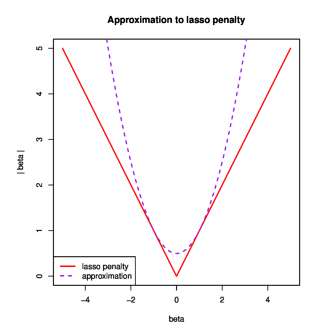
Why develop something new, when one can also make do with existing tools? The loss function of the lasso regression estimator can be optimized by iterative application of ridge regression (as pointed out in ). It requires an approximation of the lasso penalty, or the absolute value function. Set [math]p=1[/math] and let [math]\beta_0[/math] be an initial parameter value for [math]\beta[/math] around which the absolute value function [math]| \beta |[/math] is to be approximated. Its quadratic approximation then is:

[[math]] \begin{eqnarray*} |\beta | & \approx & |\beta_0 | + \tfrac{1}{2} | \beta_0 |^{-2} (\beta^2 - \beta_0^2 ). \end{eqnarray*} [[/math]]

An illustration of this approximation is provided in the left panel of Figure.

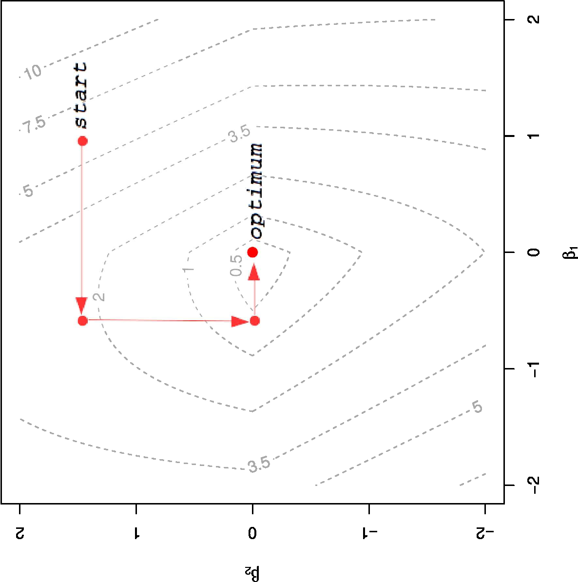
Left panel: quadratic approximation (i.e. the ridge penalty) to the absolute value function (i.e. the lasso penalty). Right panel: Illustration of the coordinate descent algorithm. The dashed grey lines are the level sets of the lasso regression loss function. The red arrows depict the parameter updates. These arrows are parallel to either the [math]\beta_1[/math] or the [math]\beta_2[/math] parameter axis, thus indicating that the regression parameter [math]\bbeta[/math] is updated coordinate-wise.

The lasso regression estimator is evaluated through iterative application of the ridge regression estimator. This iterative procedure needs initiation by some guess [math]\bbeta^{(0)}[/math] for [math]\bbeta[/math]. For example, the ridge estimator itself may serve as such. Then, at the [math]k+1[/math]-th iteration an update [math]\bbeta^{(k+1)}[/math] of the lasso regression estimator of [math]\bbeta[/math] is to be found. Application of the quadratic approximation to the absolute value functions of the elements of [math]\bbeta[/math] (around the [math]k[/math]-th update [math]\bbeta^ {(k)}[/math]) in the lasso penalty yields an approximation to the lasso regression loss function:

[[math]] \begin{eqnarray*} \| \mathbf{Y} - \mathbf{X} \, \bbeta^{(k+1)} \|^2_2 + \lambda_1 \| \bbeta^{(k+1)} \|_1 & \approx & \| \mathbf{Y} - \mathbf{X} \, \bbeta^{(k+1)} \|^2_2 + \lambda_1 \| \bbeta^{(k)} \|_1 \\ & & + \tfrac{1}{2} \lambda_1 \sum\nolimits_{j=1}^p |\beta_j^{(k)}|^{-1} [ \beta_j^{(k+1)} ]^2 - \tfrac{1}{2} \lambda_1 \sum\nolimits_{j=1}^p |\beta_j^{(k)}|^{-1} [ \beta_j^{(k)} ]^2 \\ & \propto & \| \mathbf{Y} - \mathbf{X} \, \bbeta^{(k+1)} \|^2_2 + \tfrac{1}{2} \lambda_1 \sum\nolimits_{j=1}^p |\beta_j^{(k)}|^{-1} [ \beta_j^{(k+1)} ]^2. \end{eqnarray*} [[/math]]

The loss function now contains a weighted ridge penalty. In this one recognizes a generalized ridge regression loss function (see Chapter Generalizing ridge regression ). As its minimizer is known, the approximated lasso regression loss function is optimized by:

[[math]] \begin{eqnarray*} \bbeta^{(k+1)}(\lambda_1) & = & \{ \mathbf{X}^{\top} \mathbf{X} + \lambda_1 \PPsi[ \bbeta^{(k)}(\lambda_1) ] \}^{-1} \mathbf{X}^{\top} \mathbf{Y} \end{eqnarray*} [[/math]]

where

[[math]] \begin{eqnarray*} \mbox{diag}\{ \PPsi[ \bbeta^{(k)}(\lambda_1) ] \} & = & (1/|\beta_1^{(k)}|, 1/|\beta_2^{(k)}|, \ldots, 1/|\beta_p^{(k)}|). \end{eqnarray*} [[/math]]

The thus generated sequence of updates [math]\{ \bbeta^{(k)}(\lambda_1) \}_{k=0}^{\infty}[/math] converges (under ‘nice’ conditions) to the lasso regression estimator [math]\hat{\bbeta}(\lambda_1)[/math].

A note of caution. The in-built variable selection property of the lasso regression estimator may -- for large enough choices of the penalty parameter [math]\lambda_1[/math] -- cause elements of [math]\bbeta^{(k)}(\lambda_1)[/math] to become arbitrary close to zero (or, in R exceed machine precision and thereby being effectively zero) after enough updates. Consequently, the ridge penalty parameter for the [math]j[/math]-th element of regression parameter may approach infinity, as the [math]j[/math]-th element of [math]\PPsi[ \bbeta^{(k)}(\lambda_1)][/math] equals [math]|\beta_j^{(k)}|^{-1}[/math]. To accommodate this, the iterative ridge regression algorithm for the evaluation of the lasso regression estimator requires a modification. Effectively, that amounts to the removal of [math]j[/math]-th covariate from the model all together (for its estimated regression coefficient is indistinguishable from zero). After its removal, it does not return to the set of covariates. This may be problematic if two covariates are (close to) super-collinear.

Gradient ascent

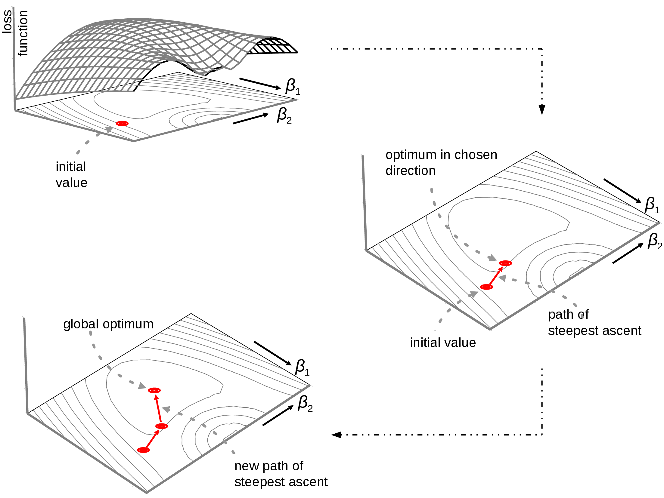
Another method of finding the lasso regression estimator and implemented in the penalized-package makes use of gradient ascent. Gradient ascent/descent is an maximization/minization method that finds the optimum of a smooth function by iteratively updating a first-order local approximation to this function. Gradient ascents runs through the following sequence of steps repetitively until convergence:

Gradient ascent

1. Choose a starting value.
2. Calculate the derivative of the function, and determine the direction in which the function increases most. This direction is the path of steepest ascent.
3. Proceed in this direction, until the function no longer increases.
4. Recalculate at this point the gradient to determine a new path of steepest ascent.
5. Repeat the above until the (region around the) optimum is found.

The procedure above is illustrated in Figure. The top panel shows the choice of the initial value. From this point the path of the steepest ascent is followed until the function no longer increases (right panel of Figure). Here the path of steepest ascent is updated along which the search for the optimum is proceeded (bottom panel of Figure).

Illustration of the gradient ascent procedure.

The use of gradient ascent to find the lasso regression estimator is frustrated by the non-differentiability (with respect to any of the regression parameters) of the lasso penalty function at zero. In this is overcome by the use of a generalized derivative. Define the directional or G\^{ateaux} derivative of the function [math]f : \mathbb{R}^p \rightarrow \mathbb{R}[/math] at [math]\mathbf{x} \in \mathbb{R}^p[/math] in the direction of [math]\mathbf{v} \in \mathbb{R}^p[/math] as:

[[math]] \begin{eqnarray*} f'(\mathbf{x}) & = & \lim_{\tau \downarrow 0} \tau^{-1} \big[ f(\mathbf{x} + \tau \mathbf{v}) - f(\mathbf{x}) \big], \end{eqnarray*} [[/math]]

assuming this limit exists. The Gâteaux derivative thus gives the infinitesimal change in [math]f[/math] at [math]\mathbf{x}[/math] in the direction of [math]\mathbf{v}[/math]. As such [math]f'(\mathbf{x})[/math] is a scalar (as is immediate from the definition when noting that [math]f(\cdot) \in \mathbb{R}[/math]) and should not be confused with the gradient (the vector of partial derivatives). Furthermore, at each point [math]\mathbf{x}[/math] there are infinitely many Gâteaux differentials (as there are infinitely many choices for [math]\mathbf{v} \in \mathbb{R}^p[/math]). In the particular case when [math]\mathbf{v} = \mathbf{e}_j[/math], [math]\mathbf{e}_j[/math] the unit vector along the axis of the [math]j[/math]-th coordinate, the directional derivative coincides with the partial derivative of [math]f[/math] in the direction of [math]x_j[/math]. Relevant for the case at hand is the absolute value function [math]f(x) = | x|[/math] with [math]x \in \mathbb{R}[/math]. Evaluation of the limits in its Gâteaux derivative yields:

[[math]] \begin{eqnarray*} f'(x) & = & \left\{ \begin{array}{lcl} \mbox{v} \frac{x}{ | x| } & \mbox{if} & x \not= 0, \\ \mbox{v} & \mbox{if} & x=0, \end{array} \right. \end{eqnarray*} [[/math]]

for any [math]\mbox{v} \in \mathbb{R} \setminus \{ 0 \}[/math]. Hence, the Gâteaux derivative of [math]| x|[/math] does exits at [math]x=0[/math]. In general, the Gâteaux differential may be uniquely defined by limiting the directional vectors [math]\mathbf{v}[/math] to i) those with unit length (i.e. [math]\| \mathbf{v} \| = 1[/math]) and ii) the direction of steepest ascent. Using the Gâteaux derivative a gradient of [math]f(\cdot)[/math] at [math]\mathbf{x} \in \mathbb{R}^p[/math] may then be defined as:

[[math]] \begin{eqnarray} \label{def:GateauxDerivative} \nabla f(\mathbf{x}) & = & \left\{ \begin{array}{lcl} f'(\mathbf{x}) \cdot \mathbf{v}_{\mbox{{\tiny opt}}} & \mbox{if} & f'(\mathbf{x}) \geq 0, \\ \mathbf{0}_{p} & \mbox{if} & f'(\mathbf{x}) \lt 0, \end{array} \right. \end{eqnarray} [[/math]]

in which [math]\mathbf{v}_{\mbox{{\tiny opt}}} = \arg \max_{\{ \mathbf{v} \, : \, \| \mathbf{v} \| = 1 \} } f'(\mathbf{x})[/math]. This is the direction of steepest ascent, [math]\mathbf{v}_{\mbox{{\tiny opt}}}[/math], scaled by Gâteaux derivative, [math]f'(\mathbf{x})[/math], in the direction of [math]\mathbf{v}_{\mbox{{\tiny opt}}}[/math].

applies the definition of the Gâteaux gradient to the lasso penalized likelihood using the direction of steepest ascent as [math]\mathbf{v}_{\mbox{{\tiny opt}}}[/math]. The resulting partial Gâteaux derivative with respect to the [math]j[/math]-th element of the regression parameter [math]\bbeta[/math] is:

[[math]] \begin{eqnarray*} \frac{\partial}{ \partial \beta_j } \mathcal{L}_{\mbox{{\tiny lasso}}}(\mathbf{Y}, \mathbf{X}; \bbeta) & = & \left\{ \begin{array}{ll} \frac{\partial}{ \partial \beta_j } \mathcal{L}(\mathbf{Y}, \mathbf{X}; \bbeta) - \lambda_1 \mbox{sign} (\beta_j) & \mbox{if} \,\, \beta_j \not= 0 \\ \frac{\partial}{ \partial \beta_j } \mathcal{L}(\mathbf{Y}, \mathbf{X}; \bbeta) - \lambda_1 \mbox{sign} \big[ \frac{\partial}{ \partial \beta_j } \mathcal{L}(Y, X; \bbeta) \big] & \mbox{if} \,\, \beta_j = 0 \mbox{ and } | \partial \mathcal{L}/ \partial \beta_j | \gt \lambda_1 \\ 0 & \mbox{otherwise}, \end{array} \right. \end{eqnarray*} [[/math]]

where [math]\partial \mathcal{L}/ \partial \beta_j = \sum_{j'=1}^p (\mathbf{X}^\top \mathbf{X})_{j', j} \beta_j - (\mathbf{X}^\top \mathbf{Y})_{j}[/math]. This can be understood through a case-by-case study. The partial derivative above is assumed to be clear for the [math]\beta_j \not= 0[/math] and the ‘otherwise’ cases. That leaves the clarification of the middle case. When [math]\beta_j = 0[/math], the direction of steepest ascent of the penalized loglikelihood points either into [math]\{ \bbeta \in \mathbb{R}^p \, : \, \beta_j \gt 0 \}[/math], or [math]\{ \bbeta \in \mathbb{R}^p \, : \, \beta_j \lt 0 \}[/math], or stays in [math]\{ \bbeta \in \mathbb{R}^p \, : \, \beta_j = 0 \}[/math]. When the direction of steepest ascent points into the positive or negative half-hyperplanes, the contribution of [math]\lambda_1 | \beta_j|[/math] to the partial Gâteaux derivative is simply [math]\lambda_1[/math] or [math]-\lambda_1[/math], respectively. Then, only when the partial derivative of the log-likelihood % in the same direction together with this contribution is larger then zero, the penalized loglikelihood improves and the direction is of steepest ascent. Similarly, the direction of steepest ascent may be restricted to [math]\{ \bbeta \in \mathbb{R}^p \, | \, \beta_j = 0 \}[/math] and the contribution of [math]\lambda_1 | \beta_j|[/math] to the partial Gâteaux derivative vanishes. Then, only if the partial derivative of the loglikelihood is positive, this direction is to be pursued for the improvement of the penalized loglikelihood.

Convergence of gradient ascent can be slow close to the optimum. This is due to its linear approximation of the function. Close to the optimum the linear term of the Taylor expansion vanishes and is dominated by the second-order quadratic term. To speed-up convergence close to the optimum the gradient ascent implementation offered by the penalized-package switches to a Newton-Raphson procedure.

Coordinate descent

Coordinate descent is another optimization algorithm that may be used to evaluate the lasso regression estimator numerically, as is done by the implemention offered via the glmnet-package. Coordinate descent, instead of following the gradient of steepest descent (as in Section Gradient ascent ), minimizes the loss function along the coordinates one-at-the-time. For the [math]j[/math]-th regression parameter this amounts to finding:

[[math]] \begin{eqnarray*} \arg \min_{\beta_j} \| \mathbf{Y} - \mathbf{X} \bbeta \|_2^2 + \lambda_1 \| \bbeta \|_1 & = & \arg \min_{\beta_j} \| \mathbf{Y} - \mathbf{X}_{\ast, \setminus j} \bbeta_{\setminus j} - \mathbf{X}_{\ast, j} \beta_{j} \|_2^2 + \lambda_1 | \beta_j |_1 \\ & = & \arg \min_{\beta_j} \| \tilde{\mathbf{Y}} - \mathbf{X}_{\ast, j} \beta_{j} \|_2^2 + \lambda_1 | \beta_j |_1, \end{eqnarray*} [[/math]]

where [math]\tilde{\mathbf{Y}} = \mathbf{Y} - \mathbf{X}_{\ast, \setminus j} \bbeta_{\setminus j}[/math]. After a simple rescaling of both [math]\mathbf{X}_{\ast, j}[/math] and [math]\beta_j[/math], the minimization of the lasso regression loss function with respect to [math]\beta_j[/math] is equivalent to one with an orthonormal design matrix. From Example it is known that the minimizer is obtained by application of the soft-threshold function to the corresponding maximum likelihood estimator (now derived from [math]\tilde{\mathbf{Y}}[/math] and [math]\mathbf{X}_j[/math]). The coordinate descent algorithm iteratively runs over the [math]p[/math] elements until convergence. The right panel of Figure provides an illustration of the coordinate descent algorithm.

Convergence of the coordinate descent algorithm to the minimum of the lasso regression loss function is warranted by the convexity of this function. At each minization step the coordinate descent algorithm yields an update of the parameter estimate that corresponds to an equal or smaller value of the loss function. It, together with the compactness of diamond-shaped parameter domain and the boundedness (from below) of the lasso regression loss function, implies that the coordinate descent algorithm converges to the minimum of this lasso regression loss function. Although convergence is assured, it may take many steps for it to be reached. In particular, when

1. two covariates are strongly collinear,
2. one of the two covariate contributes only slightly more to the response,
3. and the algorithm is initiated with the weaker explanatory covariate.

The coordinate descent algorithm will then take may iterations to replace the latter covariate by the preferred one. In such cases simultaneous updating, as is done by the gradient ascent algorithm (Section Gradient ascent ), may be preferable.

Moments

In general the moments of the lasso regression estimator appear to be unknown. In certain cases an approximation can be given. This is pointed out here. Use the quadratic approximation to the absolute value function of Section Iterative ridge and approximate the lasso regression loss function around the lasso regression estimate:

[[math]] \begin{eqnarray*} \| \mathbf{Y} - \mathbf{X} \bbeta \|_2^2 + \lambda_1 \| \bbeta \|_1 & \approx & \| \mathbf{Y} - \mathbf{X} \bbeta \|_2^2 + \tfrac{1}{2} \lambda_1 \sum\nolimits_{j=1}^p |\hat{\beta}(\lambda_1)|^{-1} \, \beta_j^2. \end{eqnarray*} [[/math]]

Optimization of the right-hand side of the preceeding display with respect to [math]\bbeta[/math] gives a ‘ridge approximation’ to the lasso estimator:

[[math]] \begin{eqnarray*} \hat{\bbeta}(\lambda_1) & \approx & \{\mathbf{X}^\top \mathbf{X} + \lambda_1 \mathbf{\Psi}[\hat{\bbeta}(\lambda_1)] \}^{-1} \mathbf{X}^\top \mathbf{Y}, \end{eqnarray*} [[/math]]

with [math](\mathbf{\Psi}[\hat{\bbeta}(\lambda_1)])_{jj} = | \hat{\beta}_j(\lambda_1) |^{-1}[/math] if [math]\hat{\beta}_j(\lambda_1) \not=0[/math]. Now use this ‘ridge approximation’ to obtain the approximation to the moments of the lasso regression estimator:

[[math]] \begin{eqnarray*} \mathbb{E} [\hat{\bbeta}(\lambda_1)] & \approx & \mathbb{E} \big( \{\mathbf{X}^\top \mathbf{X} + \lambda_1 \mathbf{\Psi}[\hat{\bbeta}(\lambda_1)] \}^{-1} \mathbf{X}^\top \mathbf{Y} \big) \, \, \, = \, \, \, \{\mathbf{X}^\top \mathbf{X} + \lambda_1 \mathbf{\Psi}[\hat{\bbeta}(\lambda_1)] \}^{-1} \mathbf{X}^\top \mathbf{X} \bbeta \end{eqnarray*} [[/math]]

and

[[math]] \begin{eqnarray*} \mbox{Var} [\hat{\bbeta}(\lambda_1)] & \approx & \mbox{Var}\big( \{\mathbf{X}^\top \mathbf{X} + \lambda_1 \mathbf{\Psi}[\hat{\bbeta}(\lambda_1)] \}^{-1} \mathbf{X}^\top \mathbf{Y} \big) \\ & = & \sigma^2 \{\mathbf{X}^\top \mathbf{X} + \lambda_1 \mathbf{\Psi}[\hat{\bbeta}(\lambda_1)] \}^{-1} \mathbf{X}^\top \mathbf{X} \{\mathbf{X}^\top \mathbf{X} + \lambda_1 \mathbf{\Psi}[\hat{\bbeta}(\lambda_1)] \}^{-1}. \end{eqnarray*} [[/math]]

These approximations can only be used when the lasso regression estimate is not sparse, which is at odds with its attractiveness. A better approximation of the variance of the lasso regression estimator can be found in , but even this becomes poor when many elements of [math]\bbeta[/math] are estimated as zero.

Although the above approximations are only crude, they indicate that the moments of the lasso regression estimator exhibit similar behaviour as those of its ridge counterpart. The (approximation of the) mean [math]\mathbb{E}[\hat{\bbeta}(\lambda_1)][/math] tends to zero as [math]\lambda_1 \rightarrow \infty[/math]. This was intuitively already expected from the form of the lasso regression loss function, in which the penalty term dominates for large [math]\lambda_1[/math] and is minimized for [math]\hat{\bbeta}(\lambda_1) = \mathbf{0}_p[/math]. This may also be understood geometrically when appealing to the equivalent constrained estimation formulation of the lasso regression estimator. The parameter constraint shrinks to zero with increasing [math]\lambda_1[/math]. Hence, so must the estimator. Similarly, the (approximation of the) variance of the lasso regression estimator vanishes as the penalty parameter [math]\lambda_1[/math] grows. Again, its loss function provides the intuition: for large [math]\lambda_1[/math] the penalty term, which does not depend on data, dominates. Or, from the perspective of the constrained estimation formulation, the parameter constraint shrinks to zero as [math]\lambda_1 \rightarrow \infty[/math]. Hence, so must the variance of the estimator, as less and less room is left for it to fluctuate.

The behaviour of the mean squared error, bias squared plus variance, of the lasso regression estimator in terms of [math]\lambda_1[/math] is hard to characterize exactly without knowledge of the quality of the approximations. In particular, does a [math]\lambda_1[/math] exists such that the MSE of the lasso regression estimator outperforms that of its maximum likelihood counterpart? Nonetheless, a first observation may be obtained from reasoning in extremis. Suppose [math]\bbeta = \mathbf{0}_p[/math], which corresponds to an empty or maximally sparse model. A large value of [math]\lambda_1[/math] then yields a zero estimate of the regression parameter: [math]\hat{\bbeta}(\lambda_1) = \mathbf{0}_p[/math]. The bias squared is thus minimized: [math]\| \hat{\bbeta}(\lambda_1) - \bbeta \|_2^2 = 0[/math]. With the bias vanished and the (approximation of the) variance decreasing in [math]\lambda_1[/math], so must the MSE decrease for [math]\lambda_1[/math] larger than some value. So, for an empty model the lasso regression estimator with a sufficiently large penalty parameter yields a better MSE than the maximum likelihood estimator. For very sparse models this property may be expected to uphold, but for non-sparse models the bias squared will have a substantial contribution to the MSE, and it is thus not obvious whether a [math]\lambda_1[/math] exists that yields a favourable MSE for the lasso regression estimator. This is investigated in silico in . The simulations presented there indicate that the MSE of the lasso regression estimator is particularly sensitive to the actual [math]\bbeta[/math]. Moreover, for a large part of the parameter space [math]\bbeta \in \mathbb{R}^p[/math] the MSE of [math]\hat{\bbeta}(\lambda_1)[/math] is behind that of the maximum likelihood estimator.

The Bayesian connection

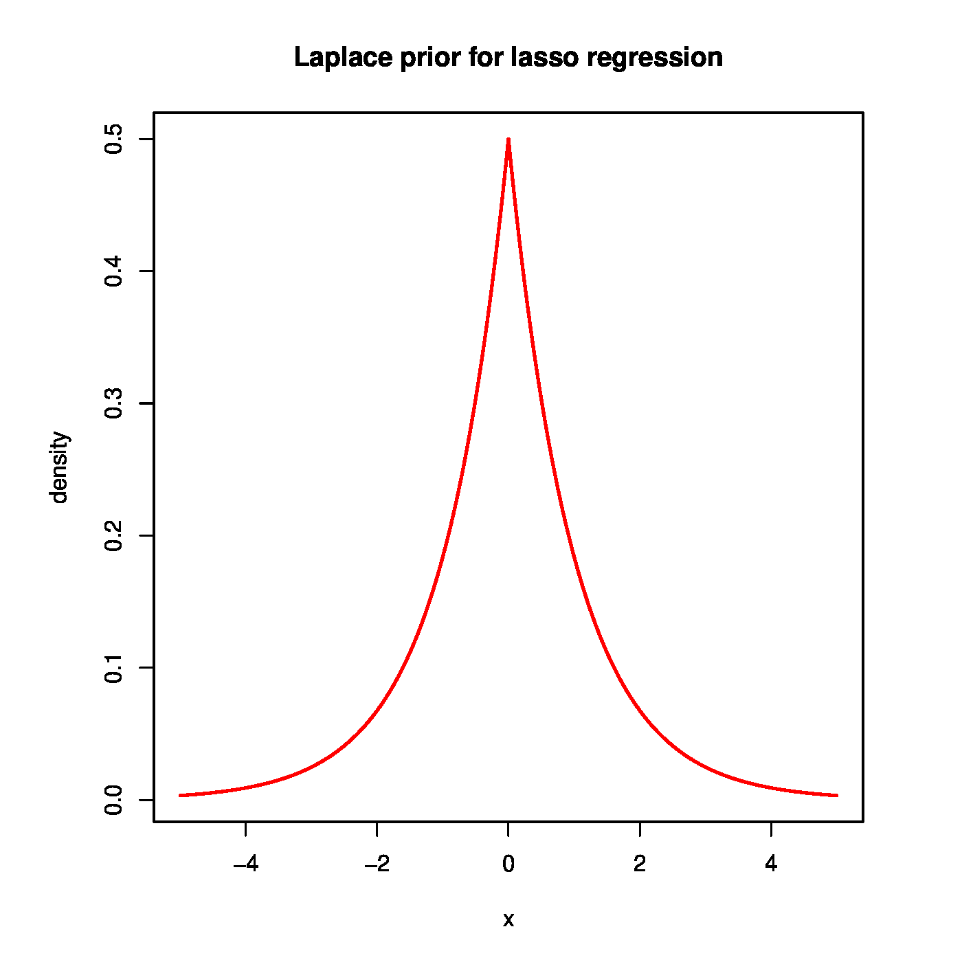
The lasso regression estimator, being a penalized estimator, knows a Bayesian formulation, much like the (generalized) ridge regression estimator could be viewed as a Bayesian estimator when imposing a Gaussian prior (cf. Chapter Bayesian regression and Section The Bayesian connection ). Instead of normal prior, the lasso regression estimator requires (as suggested by the form of the lasso penalty) a zero-centered Laplacian (or double exponential) prior for it to be viewed as a Bayesian estimator. A zero-centered Laplace distributed random variable [math]X[/math] has density [math]f_X(x) = \tfrac{1}{2} b^{-1} \exp(-|x| /b)[/math] with scale parameter [math]b \gt 0[/math]. The top panel of Figure shows the Laplace prior, and for contrast the normal prior of the ridge regression estimator. This figure reveals that the ‘lasso prior’ puts more mass close to zero and in the tails than the Gaussian ‘ridge prior’. This corroborates with the tendency of the lasso regression estimator to produce either zero or large (compared to ridge) estimates.

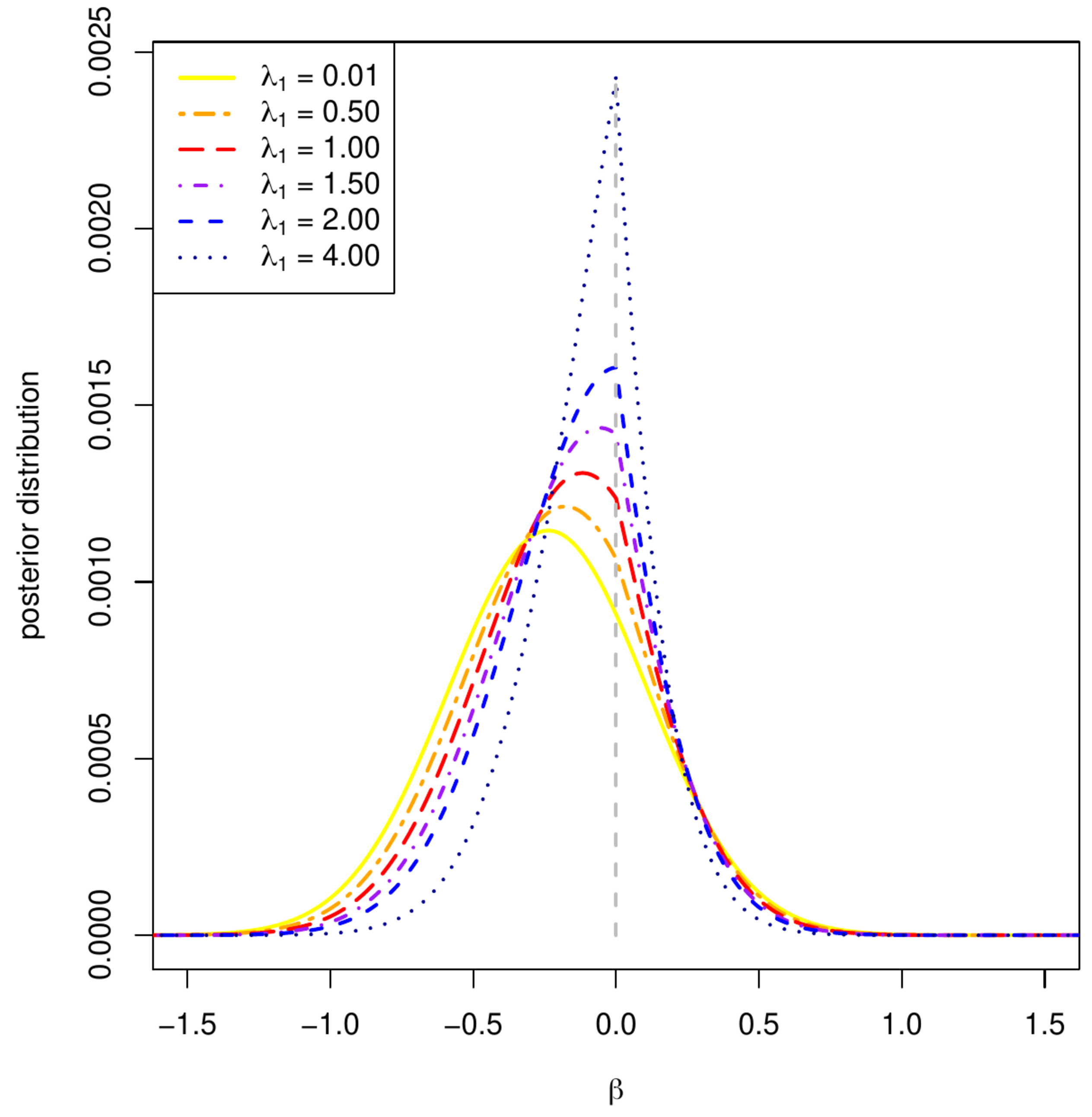
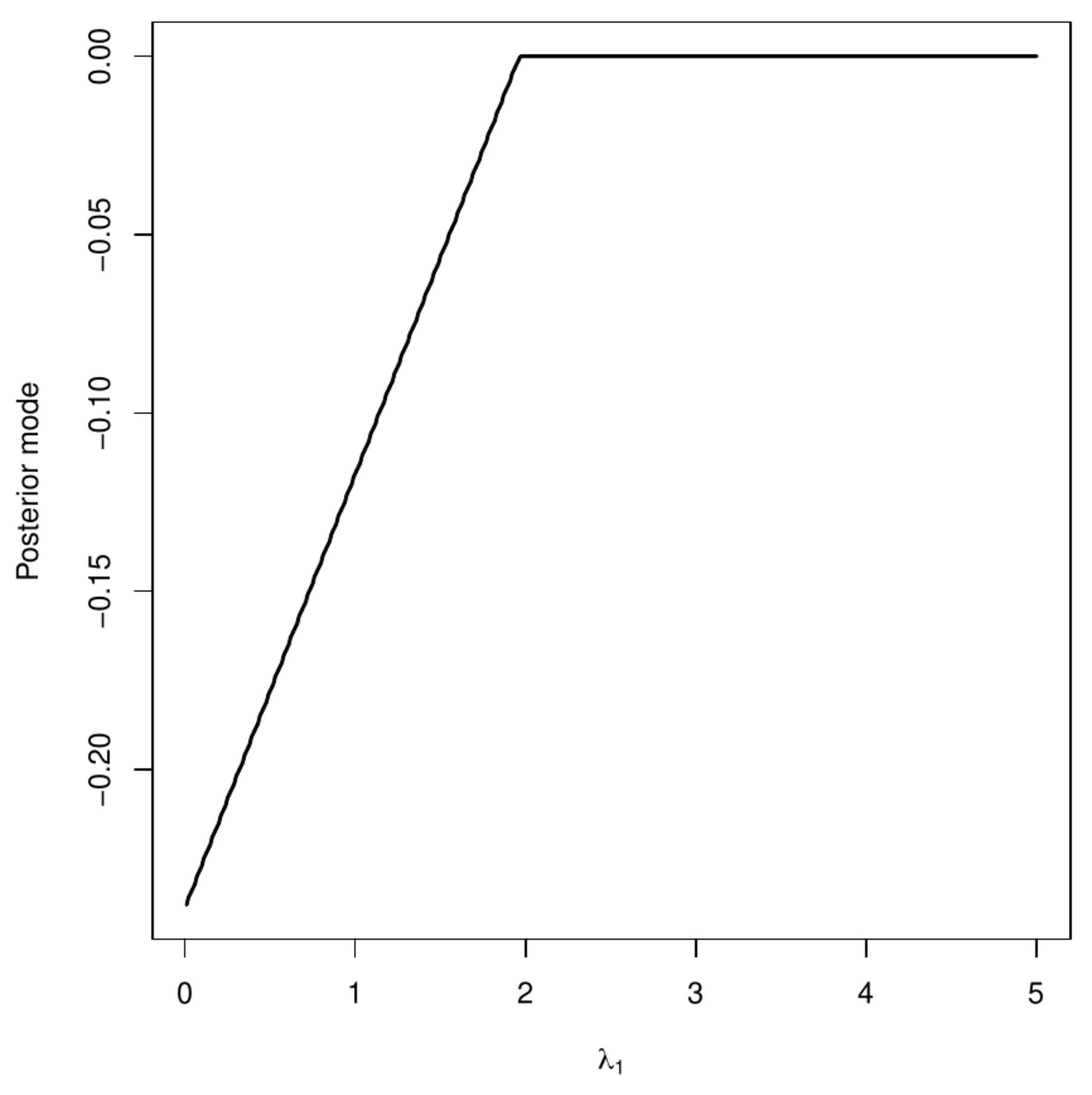
Top panel: the Laplace prior associated with the Bayesian counterpart of the lasso regression estimator. Bottom left panel: the posterior distribution of the regression parameter for various Laplace priors. Bottom right panel: posterior mode vs. the penalty parameter [math]\lambda_1[/math].

The lasso regression estimator corresponds to the maximum a posteriori (MAP) estimator of [math]\bbeta[/math], when the prior is a Laplace distribution. The posterior distribution is then proportional to:

[[math]] \begin{eqnarray*} \prod_{i=1}^n (2 \pi \sigma^2)^{-1/2} \exp [ - (2\sigma^2)^{-1} (Y_i \mathbf{X}_{i,\ast} \bbeta)^2] \times \prod_{j=1}^p (2b)^{-1} \exp( -|\beta_j |/b). \end{eqnarray*} [[/math]]

The posterior is not a well-known and characterized distribution. This is not necessary as interest concentrates here on its maximum. The location of the posterior mode coincides with the location of the maximum of logarithm of the posterior. The log-posterior is proportional to: [math]- (2\sigma^2)^{-1} \| \mathbf{Y} - \mathbf{X}\bbeta \|_2^2 - b^{-1} \| \bbeta \|_1[/math], with its maximizer minimizing [math]\| \mathbf{Y} - \mathbf{X}\bbeta \|_2^2 + (2 \sigma^2 / b) \| \bbeta \|_1[/math]. In this one recognizes the form of the lasso regression loss function. It is thus clear that the scale parameter of the Laplace distribution reciprocally relates to lasso penalty parameter [math]\lambda_1[/math], similar to the relation of the ridge penalty parameter [math]\lambda_2[/math] and the variance of the Gaussian prior of the ridge regression estimator.

The posterior may not be a standard distribution, in the univariate case ([math]p=1[/math]) it can be visualized. Specifically, the behaviour of the MAP can then be illustrated, which -- as the MAP estimator corresponds to the lasso regression estimator -- should also exhibit the selection property. The bottom left panel of Figure shows the posterior distribution for various choices of the Laplace scale parameter (i.e. lasso penalty parameter). Clearly, the mode shifts towards zero as the scale parameter decreases / lasso penalty parameter increases. In particular, the posterior obtained from the Laplace prior with the smallest scale parameter (i.e. largest penalty parameter [math]\lambda_1[/math]), although skewed to the left, has a mode placed exactly at zero. The Laplace prior may thus produce MAP estimators that select. However, for smaller values of the lasso penalty parameter the Laplace prior is not concentrated enough around zero and the contribution of the likelihood in the posterior outweighs that of the prior. The mode is then not located at zero and the parameter is ‘selected’ by the MAP estimator. The bottom right panel of Figure plots the mode of the normal-Laplace posterior vs. the Laplace scale parameter. In line with Theorem it is piece-wise linear.

go beyond the elementary correspondence of the frequentist lasso estimator and the Bayesian posterior mode and formulate the Bayesian lasso regression model. To this end they exploit the fact that the Laplace distribution can be written as a scale mixture of normal distributions with an exponentional mixing density. This allows the construction of a Gibbs sampler for the Bayesian lasso estimator. Finally, they suggest to impose a gamma-type hyperprior on the (square of the) lasso penalty parameter. Such a full Bayesian formulation of the lasso problem enables the construction of credible sets (i.e. the Bayesian counterpart of confidence intervals) to express the uncertainty of the maximum a posterior estimator. However, the lasso regression estimator may be seen as a Bayesian estimator, in the sense that it coincides with the posterior mode, the ‘lasso’ posterior distribution cannot be blindly used for uncertainty quantification. In high-dimensional sparse settings the ‘lasso’ posterior distribution of [math]\bbeta[/math] need not concentrate around the true parameter, even though its mode is a good estimator of the regression parameter (cf. Section 3 and Theorem 7 of ).

General References

van Wieringen, Wessel N. (2021). "Lecture notes on ridge regression". arXiv:1509.09169 [stat.ME].

References

- Tibshirani, R. (1996).Regularized shrinkage and selection via the lasso.Journal of the Royal Statistical Society B, 58(1), 267--288
- Bertsekas, D. P. (2014).Constrained Optimization and Lagrange Multiplier Methods.Academic press
- Fan, J. and Li, R. (2001).Variable selection via nonconcave penalized likelihood and its oracle properties.Journal of the American statistical Association, 96(456), 1348--1360
- 4.0 4.1 4.2 Goeman, J. J. (2010).[math]L_1[/math] penalized estimation in the Cox proportional hazards model.Biometrical Journal, 52, 70--84
- Osborne, M. R., Presnell, B., and Turlach, B. A. (2000).On the lasso and its dual.Journal of Computational and Graphical Statistics, 9(2), 319--337
- Hansen, B. E. (2015).The risk of James--Stein and lasso shrinkage.Econometric Reviews, 35(8-10), 1456--1470
- Park, T. and Casella, G. (2008).The Bayesian lasso.Journal of the American Statistical Association, 103(482), 681--686
- Castillo, I., Schmidt-Hieber, J., and Van der Vaart, A. W. (2015).Bayesian linear regression with sparse priors.The Annals of Statistics, 43(5), 1986--2018