guide:1a3054fd98: Difference between revisions
mNo edit summary |
mNo edit summary |
||
| (3 intermediate revisions by the same user not shown) | |||
| Line 47: | Line 47: | ||
which comprises a weighted least squares criterion and a generalized ridge penalty. In this <math>\mathbf{W}</math> is a <math>(n \times n)</math>-dimensional, diagonal matrix with <math>(\mathbf{W})_{ii} \in [0,1]</math> representing the weight of the <math>i</math>-th observation. The penalty is now a quadratic form with penalty parameter <math>\mathbf{\Delta}</math>, a <math>(p \times p)</math>-dimensional, positive definite, symmetric matrix. When <math>\mathbf{\Delta} = \lambda \mathbf{I}_{pp}</math>, one regains the spherical penalty of ‘regular ridge regression’. This penalty shrinks each element of the regression parameter <math>\bbeta</math> equally along the unit vectors <math>\mathbf{e}_j</math>. Generalizing <math>\mathbf{\Delta}</math> to the class of symmetric, positive definite matrices <math>\mathcal{S}_{++}</math> allows for ''i)'' different penalization per regression parameter, and ''ii)'' joint (or correlated) shrinkage among the elements of <math>\bbeta</math>. The penalty parameter <math>\mathbf{\Delta}</math> determines the speed and direction of shrinkage. The <math>p</math>-dimensional column vector <math>\bbeta_0</math> is a user-specified, non-random target towards which <math>\bbeta</math> is shrunken as the penalty parameter increases. When recasting generalized ridge estimation as a constrained estimation problem, the implications of the penalty may be visualized ([[#fig:generalizedRidgeIllustration|Figure]], left panel). The generalized ridge penalty is a quadratic form centered around <math>\bbeta_0</math>. In [[#fig:generalizedRidgeIllustration|Figure]] the parameter constraint clearly is ellipsoidal (and not spherical). Moreover, the center of this ellipsoid is not at zero. | which comprises a weighted least squares criterion and a generalized ridge penalty. In this <math>\mathbf{W}</math> is a <math>(n \times n)</math>-dimensional, diagonal matrix with <math>(\mathbf{W})_{ii} \in [0,1]</math> representing the weight of the <math>i</math>-th observation. The penalty is now a quadratic form with penalty parameter <math>\mathbf{\Delta}</math>, a <math>(p \times p)</math>-dimensional, positive definite, symmetric matrix. When <math>\mathbf{\Delta} = \lambda \mathbf{I}_{pp}</math>, one regains the spherical penalty of ‘regular ridge regression’. This penalty shrinks each element of the regression parameter <math>\bbeta</math> equally along the unit vectors <math>\mathbf{e}_j</math>. Generalizing <math>\mathbf{\Delta}</math> to the class of symmetric, positive definite matrices <math>\mathcal{S}_{++}</math> allows for ''i)'' different penalization per regression parameter, and ''ii)'' joint (or correlated) shrinkage among the elements of <math>\bbeta</math>. The penalty parameter <math>\mathbf{\Delta}</math> determines the speed and direction of shrinkage. The <math>p</math>-dimensional column vector <math>\bbeta_0</math> is a user-specified, non-random target towards which <math>\bbeta</math> is shrunken as the penalty parameter increases. When recasting generalized ridge estimation as a constrained estimation problem, the implications of the penalty may be visualized ([[#fig:generalizedRidgeIllustration|Figure]], left panel). The generalized ridge penalty is a quadratic form centered around <math>\bbeta_0</math>. In [[#fig:generalizedRidgeIllustration|Figure]] the parameter constraint clearly is ellipsoidal (and not spherical). Moreover, the center of this ellipsoid is not at zero. | ||
<div class="d-flex justify-content-center" | <div class="d-flex justify-content-center flex-column flex-md-row" id="fig:generalizedRidgeIllustration"> | ||
[[File:generalizedRidgeIllustration_penalty.png | 400px]] | |||
[[File:generalizedRidgeIllustration_penalty.png | 400px | [[File:generalizedRidgeIllustration_paths.png | 400px ]] | ||
</div> | </div> | ||
<div class="figure-caption"> | |||
Left panel: the contours of the likelihood (grey solid ellipsoids) and the parameter constraint implied by the generalized penalty (black dashed ellipsoids) Right panel: generalized (fat coloured lines) and ‘regular’ (thin coloured lines) regularization paths of four regression coefficients. The dotted grey (straight) lines indicated the targets towards the generalized ridge penalty shrinks regression coefficient estimates. | |||
</div> | |||
The addition of the generalized ridge penalty to the sum-of-squares ensures the existence of a unique regression estimator in the face of super-collinearity. The generalized penalty is a non-degenerated quadratic form in <math>\bbeta</math> due to the positive definiteness of the matrix <math>\mathbf{\Delta}</math>. As it is non-degenerate, it is strictly convex. Consequently, the generalized ridge regression loss function (\ref{form:generalizedRidgeLoss}), being the sum of a convex and strictly convex function, is also strictly convex. This warrants the existence of a unique global minimum and, thereby, a unique estimator. | The addition of the generalized ridge penalty to the sum-of-squares ensures the existence of a unique regression estimator in the face of super-collinearity. The generalized penalty is a non-degenerated quadratic form in <math>\bbeta</math> due to the positive definiteness of the matrix <math>\mathbf{\Delta}</math>. As it is non-degenerate, it is strictly convex. Consequently, the generalized ridge regression loss function (\ref{form:generalizedRidgeLoss}), being the sum of a convex and strictly convex function, is also strictly convex. This warrants the existence of a unique global minimum and, thereby, a unique estimator. | ||
| Line 113: | Line 117: | ||
To illustrate the effect of the fused ridge penalty on the estimation of the linear regression model <math>\mathbf{Y} = \mathbf{X} \bbeta + \vvarepsilon</math>, let <math>\beta_j = \phi_{0,1}(z_j)</math> with <math>z_j =-30 + \tfrac{6}{50} j</math> for <math>j=1, \ldots, 500</math>. Sample the elements of the design matrix <math>\mathbf{X}</math> and those of the error vector <math>\vvarepsilon</math> from the standard normal distribution, then form the response <math>\mathbf{Y}</math> from the linear model. The regression parameter is estimated through fused ridge loss minimization with <math>\lambda=1000</math>. The estimate is shown in the left panel of [[#fig:fusedRidgeIllustration|Figure]] (red line). For reference the figure includes the true <math>\bbeta</math> (black line) and the ‘regular ridge’ estimate with <math>\lambda=1</math> (blue line). Clearly, the fused ridge estimate yields a nice smooth vector of <math>\bbeta</math> estimates | To illustrate the effect of the fused ridge penalty on the estimation of the linear regression model <math>\mathbf{Y} = \mathbf{X} \bbeta + \vvarepsilon</math>, let <math>\beta_j = \phi_{0,1}(z_j)</math> with <math>z_j =-30 + \tfrac{6}{50} j</math> for <math>j=1, \ldots, 500</math>. Sample the elements of the design matrix <math>\mathbf{X}</math> and those of the error vector <math>\vvarepsilon</math> from the standard normal distribution, then form the response <math>\mathbf{Y}</math> from the linear model. The regression parameter is estimated through fused ridge loss minimization with <math>\lambda=1000</math>. The estimate is shown in the left panel of [[#fig:fusedRidgeIllustration|Figure]] (red line). For reference the figure includes the true <math>\bbeta</math> (black line) and the ‘regular ridge’ estimate with <math>\lambda=1</math> (blue line). Clearly, the fused ridge estimate yields a nice smooth vector of <math>\bbeta</math> estimates | ||
<div class="d-flex justify-content-center"> | |||
< | <div id="fig:fusedRidgeIllustration"> | ||
[[File: | <div class="d-flex flex-column flex-md-row justify-content-center"> | ||
[[File:fusedRidgeIllustration_simulation.png | 400px ]] | |||
[[File:effectHomogeneityPenalty.png | 400px ]] | |||
</div> | |||
<div class="d-flex flex-column flex-md-row justify-content-center"> | |||
[[File:effectCodataPenalty.png | 400px ]] | |||
[[File:fusedRidge_KRASexample.png | 400px ]] | |||
</div> | |||
</div> | |||
<div class="figure-caption"> | |||
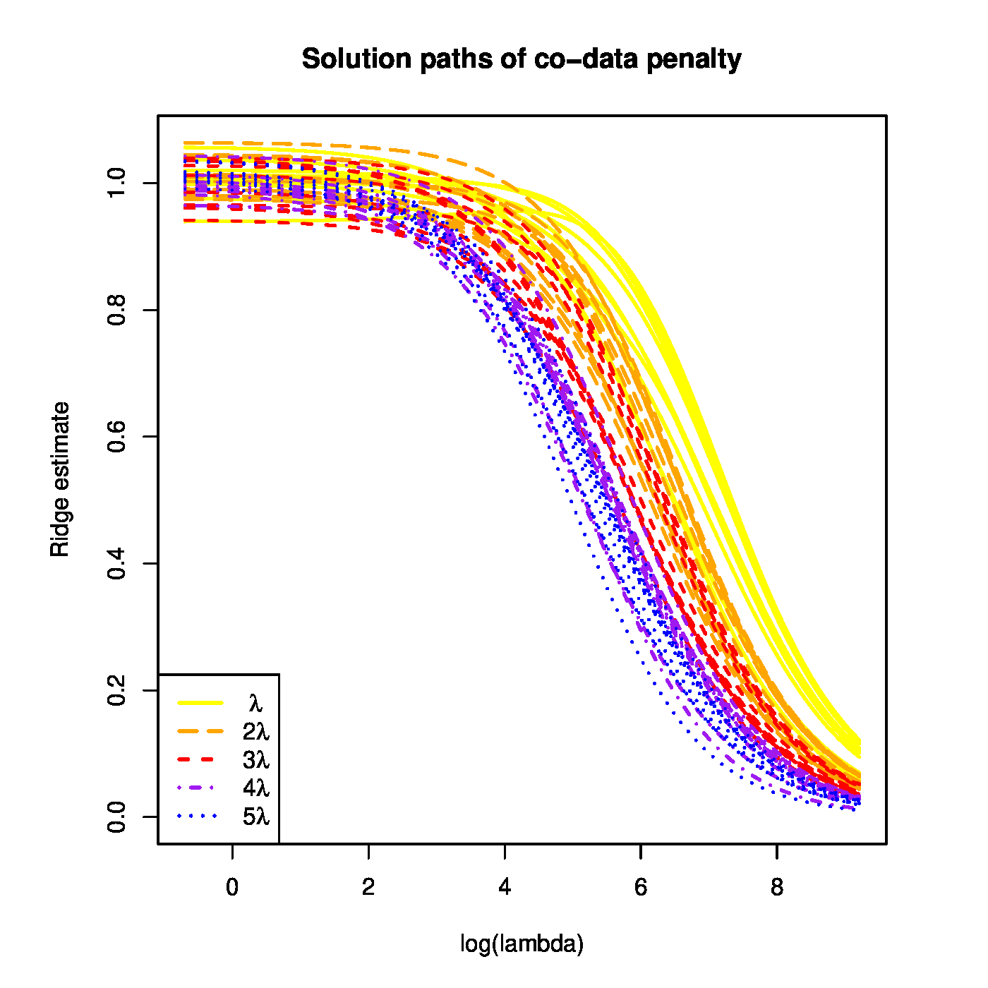
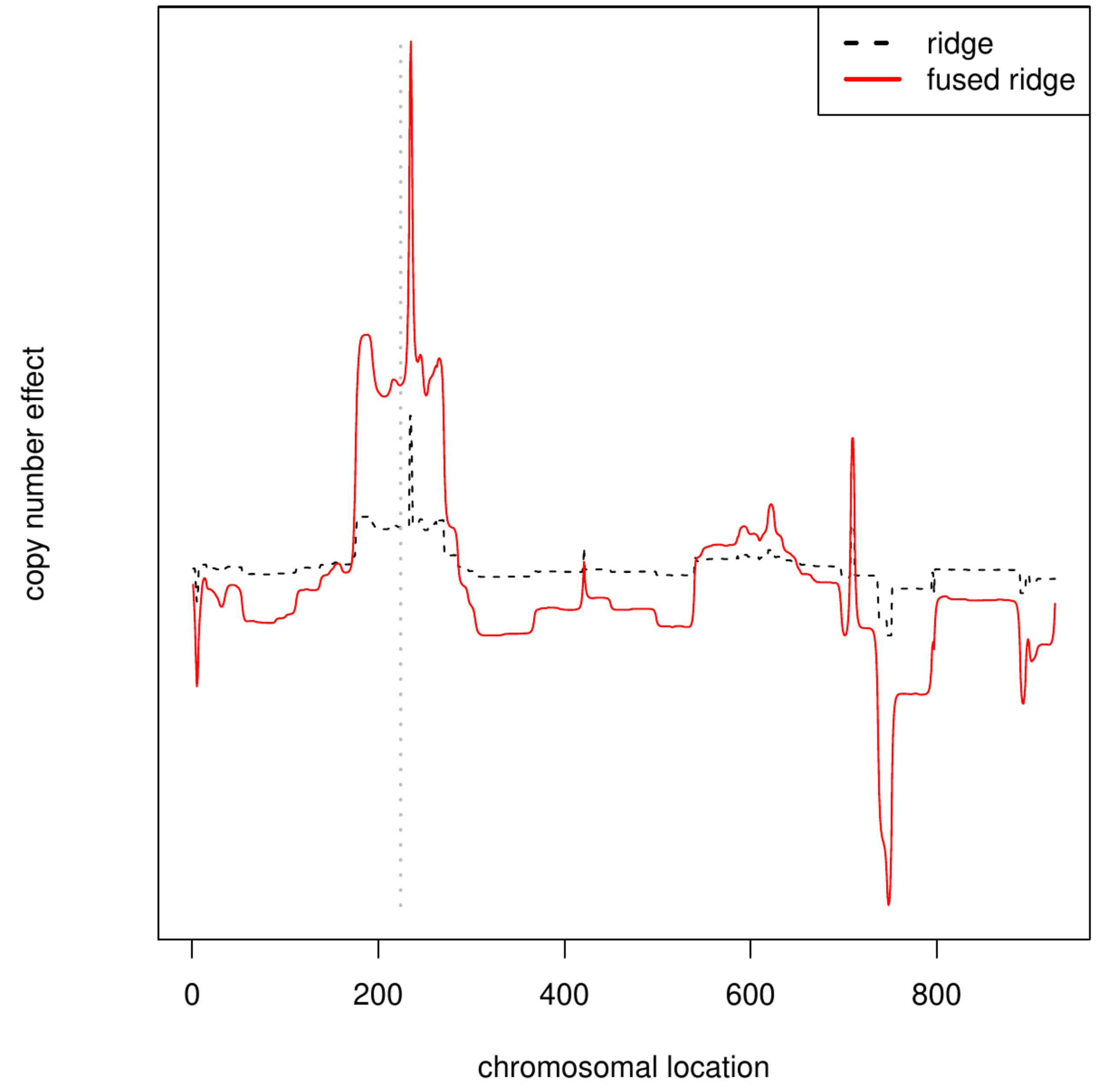
Top left panel: illustration of the fused ridge estimator (in simulation). The true parameter <math>\bbeta</math> and its ridge and fused ridge estimates against their spatial order. Top right panel: regularization path of the ridge regression estimator with a ‘homogeneity’ penalty matrix. Bottom left panel: regularization path of the ridge regression estimator with a ‘co-data’ penalty matrix. Bottom right panel: Ridge vs. fused ridge estimates of the DNA copy effect on KRAS expression levels. The dashed, grey vertical bar indicates the location of the KRAS gene. | |||
</div> | </div> | ||
'''Example''' (A ‘ridge to homogeneity’) | '''Example''' (A ‘ridge to homogeneity’) | ||
| Line 204: | Line 220: | ||
==<span id="sect:genRidgeBayes"></span>The Bayesian connection== | ==<span id="sect:genRidgeBayes"></span>The Bayesian connection== | ||
This generalized ridge regression estimator can, like the regular ridge regression estimator, be viewed as a Bayesian estimator. It requires to replace the conjugate prior on <math>\bbeta</math> by a more general normal law, <math>\bbeta \sim \mathcal{N}(\bbeta_0, \sigma^2 \mathbf{\Delta}^{-1})</math>, but retains the inverse gamma prior on <math>\sigma^2</math>. The joint posterior distribution of <math>\bbeta</math> and <math>\sigma^2</math> is then obtained analogously to the derivation of posterior with a standard normal prior on <math>\bbeta</math> as presented in Chapter [[guide:52e4430d25 | Bayesian regression ]] (the details are left as | This generalized ridge regression estimator can, like the regular ridge regression estimator, be viewed as a Bayesian estimator. It requires to replace the conjugate prior on <math>\bbeta</math> by a more general normal law, <math>\bbeta \sim \mathcal{N}(\bbeta_0, \sigma^2 \mathbf{\Delta}^{-1})</math>, but retains the inverse gamma prior on <math>\sigma^2</math>. The joint posterior distribution of <math>\bbeta</math> and <math>\sigma^2</math> is then obtained analogously to the derivation of posterior with a standard normal prior on <math>\bbeta</math> as presented in Chapter [[guide:52e4430d25 | Bayesian regression ]] (the details are left as [[exercise:0705fd77a7|Exercise]]): | ||
<math display="block"> | <math display="block"> | ||
| Line 226: | Line 242: | ||
This implies <math>\mathbb{E}(\bbeta \, | \, \sigma^2, \mathbf{Y}, \mathbf{X}) = \hat{\bbeta}(\mathbf{\Delta})</math>. Hence, the generalized ridge regression estimator too can be viewed as the Bayesian posterior mean estimator of <math>\bbeta</math> when imposing a multivariate Gaussian prior on the regression parameter. | This implies <math>\mathbb{E}(\bbeta \, | \, \sigma^2, \mathbf{Y}, \mathbf{X}) = \hat{\bbeta}(\mathbf{\Delta})</math>. Hence, the generalized ridge regression estimator too can be viewed as the Bayesian posterior mean estimator of <math>\bbeta</math> when imposing a multivariate Gaussian prior on the regression parameter. | ||
The Bayesian formulation of our generalization of ridge regression provides additional intuition of the penalty parameters <math>\bbeta_0</math> and <math>\mathbf{\Delta}</math>. For instance, a better initial guess, i.e. <math>\bbeta_0</math>, yields a better posterior mean and mode. Or, less uncertainty in the prior, i.e. a smaller (in the positive definite ordering sense) variance <math>\mathbf{\Delta}</math>, yields a more concentrated posterior. These claims are underpinned in | The Bayesian formulation of our generalization of ridge regression provides additional intuition of the penalty parameters <math>\bbeta_0</math> and <math>\mathbf{\Delta}</math>. For instance, a better initial guess, i.e. <math>\bbeta_0</math>, yields a better posterior mean and mode. Or, less uncertainty in the prior, i.e. a smaller (in the positive definite ordering sense) variance <math>\mathbf{\Delta}</math>, yields a more concentrated posterior. These claims are underpinned in [[exercise:3c9a764dd4 |Question]]. The intuition they provide guides in the choice of penalty parameters <math>\bbeta_0</math> and <math>\mathbf{\Delta}</math>. | ||
==Application== | ==Application== | ||
Latest revision as of 09:53, 6 July 2023
[math] \require{textmacros} \require{html} \def \bbeta {\bf \beta} \def\fat#1{\mbox{\boldmath$#1$}} \def\reminder#1{\marginpar{\rule[0pt]{1mm}{11pt}}\textbf{#1}} \def\SSigma{\bf \Sigma} \def\ttheta{\bf \theta} \def\aalpha{\bf \alpha} \def\bbeta{\bf \beta} \def\ddelta{\bf \delta} \def\eeta{\bf \eta} \def\llambda{\bf \lambda} \def\ggamma{\bf \gamma} \def\nnu{\bf \nu} \def\vvarepsilon{\bf \varepsilon} \def\mmu{\bf \mu} \def\nnu{\bf \nu} \def\ttau{\bf \tau} \def\SSigma{\bf \Sigma} \def\TTheta{\bf \Theta} \def\XXi{\bf \Xi} \def\PPi{\bf \Pi} \def\GGamma{\bf \Gamma} \def\DDelta{\bf \Delta} \def\ssigma{\bf \sigma} \def\UUpsilon{\bf \Upsilon} \def\PPsi{\bf \Psi} \def\PPhi{\bf \Phi} \def\LLambda{\bf \Lambda} \def\OOmega{\bf \Omega} [/math]
The exposé on ridge regression may be generalized in many ways. Among others different generalized linear models may be considered (confer Section Ridge estimation ). In this section we stick to the linear regression model [math]\mathbf{Y} = \mathbf{X} \bbeta + \vvarepsilon[/math] with the usual assumptions, but fit it in weighted fashion and generalize the common, spherical penalty. The loss function corresponding to this scenario is:
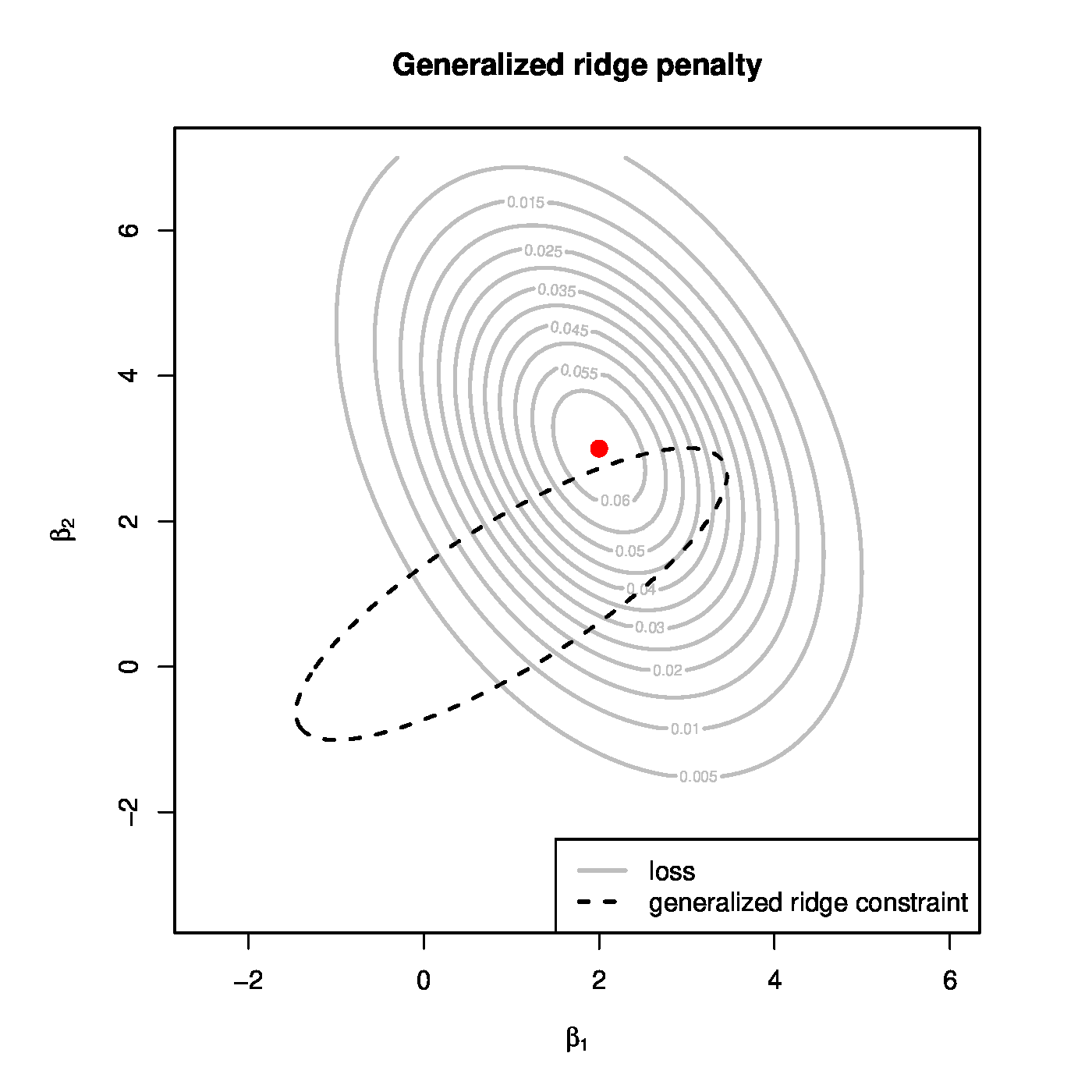
which comprises a weighted least squares criterion and a generalized ridge penalty. In this [math]\mathbf{W}[/math] is a [math](n \times n)[/math]-dimensional, diagonal matrix with [math](\mathbf{W})_{ii} \in [0,1][/math] representing the weight of the [math]i[/math]-th observation. The penalty is now a quadratic form with penalty parameter [math]\mathbf{\Delta}[/math], a [math](p \times p)[/math]-dimensional, positive definite, symmetric matrix. When [math]\mathbf{\Delta} = \lambda \mathbf{I}_{pp}[/math], one regains the spherical penalty of ‘regular ridge regression’. This penalty shrinks each element of the regression parameter [math]\bbeta[/math] equally along the unit vectors [math]\mathbf{e}_j[/math]. Generalizing [math]\mathbf{\Delta}[/math] to the class of symmetric, positive definite matrices [math]\mathcal{S}_{++}[/math] allows for i) different penalization per regression parameter, and ii) joint (or correlated) shrinkage among the elements of [math]\bbeta[/math]. The penalty parameter [math]\mathbf{\Delta}[/math] determines the speed and direction of shrinkage. The [math]p[/math]-dimensional column vector [math]\bbeta_0[/math] is a user-specified, non-random target towards which [math]\bbeta[/math] is shrunken as the penalty parameter increases. When recasting generalized ridge estimation as a constrained estimation problem, the implications of the penalty may be visualized (Figure, left panel). The generalized ridge penalty is a quadratic form centered around [math]\bbeta_0[/math]. In Figure the parameter constraint clearly is ellipsoidal (and not spherical). Moreover, the center of this ellipsoid is not at zero.
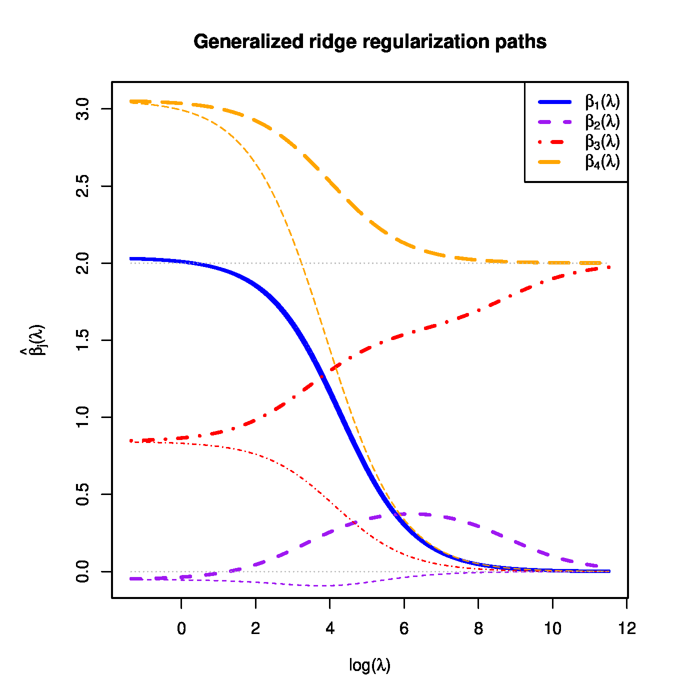
Left panel: the contours of the likelihood (grey solid ellipsoids) and the parameter constraint implied by the generalized penalty (black dashed ellipsoids) Right panel: generalized (fat coloured lines) and ‘regular’ (thin coloured lines) regularization paths of four regression coefficients. The dotted grey (straight) lines indicated the targets towards the generalized ridge penalty shrinks regression coefficient estimates.
The addition of the generalized ridge penalty to the sum-of-squares ensures the existence of a unique regression estimator in the face of super-collinearity. The generalized penalty is a non-degenerated quadratic form in [math]\bbeta[/math] due to the positive definiteness of the matrix [math]\mathbf{\Delta}[/math]. As it is non-degenerate, it is strictly convex. Consequently, the generalized ridge regression loss function (\ref{form:generalizedRidgeLoss}), being the sum of a convex and strictly convex function, is also strictly convex. This warrants the existence of a unique global minimum and, thereby, a unique estimator.
Like for the ‘regular’ (ridge loss function), there is an explicit expression for the optimum of the generalized ridge loss function (\ref{form:generalizedRidgeLoss}). To see this, obtain the estimating equation of [math]\bbeta[/math] through equating its derivative with respect to [math]\bbeta[/math] to zero:
This is solved by:
Clearly, this reduces to the ‘regular’ ridge regression estimator by setting [math]\mathbf{W} = \mathbf{I}_{nn}[/math], [math]\bbeta_0 = \mathbf{0}_{p}[/math], and [math]\mathbf{\Delta} = \lambda \mathbf{I}_{pp}[/math]. The effects of the generalized ridge penalty on the coefficients of corresponding estimator can be seen in the regularization paths of the estimator's coefficients. Figure (right panel) contains an example of the regularization paths for coefficients of a linear regression model with four explanatory variables. Most striking is the limiting behaviour of the estimates of [math]\beta_3[/math] and [math]\beta_4[/math] for large values of the penalty parameter [math]\lambda[/math]: they convergence to a non-zero value (as was specified by a nonzero [math]\beta_0[/math]). More subtle is the (temporary) convergence of the regularization paths of the estimates of [math]\beta_2[/math] and [math]\beta_3[/math]. That of [math]\beta_2[/math] is pulled away from zero (its true value and approximately its unpenalized estimate) towards the estimate of [math]\beta_3[/math]. In the regularization path of [math]\beta_3[/math] this can be observed in a delayed convergence to its nonzero target value (for comparison consider that of [math]\beta_4[/math]). For reference the corresponding regularization paths of the ‘regular’ ridge estimates (as thinner lines of the same colour) are included in Figure.
Example (Fused ridge estimation)
An example of a generalized ridge penalty is the fused ridge penalty (as introduced by [1]). Consider the standard linear model [math]\mathbf{Y} = \mathbf{X} \bbeta + \vvarepsilon[/math]. The fused ridge estimator of [math]\bbeta[/math] then minimizes:
The penalty in the loss function above can be written as a generalized ridge penalty:
The matrix [math]\mathbf{\Delta}[/math] employed above is semi-positive definite and therefore the loss function (\ref{form:fusedRidgeLoss}) need not be strictly convex. Hence, often a regular ridge penalty [math]\| \bbeta \|_2^2[/math] is added (with its own penalty parameter).
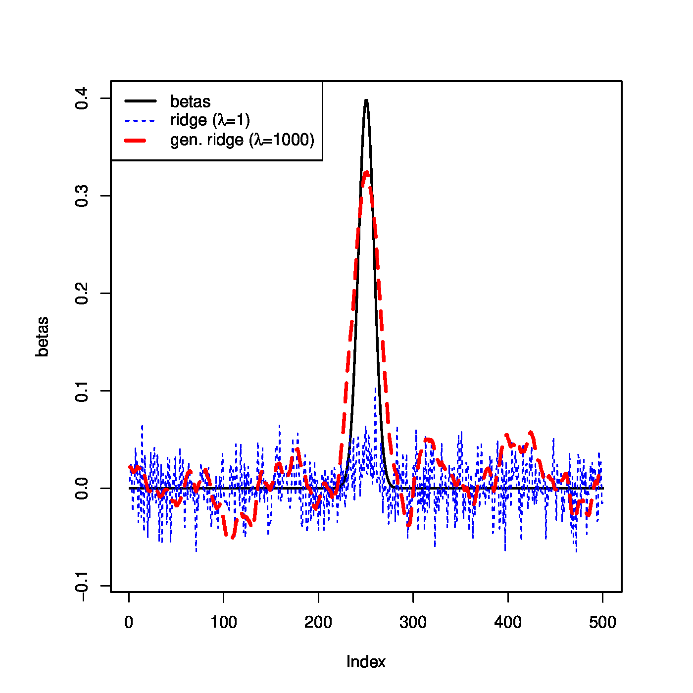
To illustrate the effect of the fused ridge penalty on the estimation of the linear regression model [math]\mathbf{Y} = \mathbf{X} \bbeta + \vvarepsilon[/math], let [math]\beta_j = \phi_{0,1}(z_j)[/math] with [math]z_j =-30 + \tfrac{6}{50} j[/math] for [math]j=1, \ldots, 500[/math]. Sample the elements of the design matrix [math]\mathbf{X}[/math] and those of the error vector [math]\vvarepsilon[/math] from the standard normal distribution, then form the response [math]\mathbf{Y}[/math] from the linear model. The regression parameter is estimated through fused ridge loss minimization with [math]\lambda=1000[/math]. The estimate is shown in the left panel of Figure (red line). For reference the figure includes the true [math]\bbeta[/math] (black line) and the ‘regular ridge’ estimate with [math]\lambda=1[/math] (blue line). Clearly, the fused ridge estimate yields a nice smooth vector of [math]\bbeta[/math] estimates
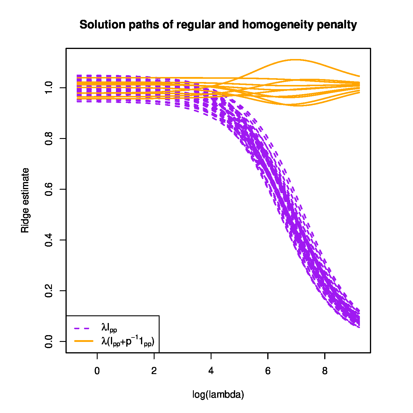
Top left panel: illustration of the fused ridge estimator (in simulation). The true parameter [math]\bbeta[/math] and its ridge and fused ridge estimates against their spatial order. Top right panel: regularization path of the ridge regression estimator with a ‘homogeneity’ penalty matrix. Bottom left panel: regularization path of the ridge regression estimator with a ‘co-data’ penalty matrix. Bottom right panel: Ridge vs. fused ridge estimates of the DNA copy effect on KRAS expression levels. The dashed, grey vertical bar indicates the location of the KRAS gene.
Example (A ‘ridge to homogeneity’)
A different form of fusion proposed by [2] shrinks (a subset of) the regression parameters to a common value. In the work of [2] this common value is the mean of these regression parameters. This mean is also learned from data, alongside to individual elements of regression parameter. Hereto the sum-of-squares is augmented by the following penalty:
Straightforward application of this penalty within the context of the linear regression model may seem farfetched. That is, why would a common effect of all covariates be desirable? Indeed, the motivation of [2] stems from a different context. Translated to the present standard linear regression model context, that motivation could be thought of -- loosely -- as an application of the penalty (\ref{form.homogeneityPenalty}) to subsets of the regression parameter. Situations arise where many covariates are only slightly different operationalizations of the same trait. For instance, in brain image data the image itself is often summarized in many statistics virtually measuring the same thing. In extremis, those could be the mean, median and trimmed mean of the intensity of a certain region of the image. It would be ridiculous to assume these three summary statistics to have a wildly different effect, and shrinkage to a common value seems sensible practice. Finally, note that the above employed penalty matrix, [math]\mathbf{\Delta} = \lambda ( \mathbf{I}_{pp} - p^{-1} \mathbf{1}_{pp})[/math], is nonnegative definite. Hence, in the face of (super-) collinearity, an additional penalty terms is required for a well-defined estimator.
We illustrate the effect of the ‘homogeneity’ penalty (\ref{form.homogeneityPenalty}). We sample from the linear regression model [math]\mathbf{Y} = \mathbf{X} \bbeta + \vvarepsilon[/math] with [math]\bbeta = \mathbf{1}_{50}[/math] and both the elements of the design matrix as well as the error sampled from the standard normal distribution. We then evaluate the regularization path of the estimator (\ref{form:generalizedRidgeEstimator}) with [math]\mathbf{\Delta}[/math] a diagonal [math]2 \times 2[/math] block matrix. The first diagonal block [math]\mathbf{\Delta}_{11} = \lambda (\mathbf{I}_{10, 10} - \tfrac{1}{10} \mathbf{1}_{10,10})[/math] and the second [math]\mathbf{\Delta}_{22} = \lambda \mathbf{I}_{40, 40}[/math]. The resulting regularization paths are shown in the top right panel of Figure
Example (Co-data)
Another utilization of the generalized ridge regression estimator (\ref{form:generalizedRidgeEstimator}) can be found in applications where groups of covariates are deemed to be differentially important for the explaination of the response. [3] suggests to form these groups on the basis of co-data. The co-data concept refers to auxillary data on the covariates not necessary directly related to but possibly implicitly informative for the to-be-estimated model. For instance, for each covariate a marginal [math]p[/math]-value or effect estimate from a different study may be available. The covariate groups may then be formed on the basis of the size of this statistic. Alternatively, co-data may comprise some form of biological annotation, e.g. pathway membership of genes. Irrespectively, a shared group membership of covariates is indicative of an equal (implicit) relevance for model fitting. The possible importance differences among the covariate groups are accommodated through the augmentation of the loss by a sum of group-wise regular ridge penalties. That is, the elements of the regression parameter that correspond to the covariates of the same group are penalized by the sum of the square of these elements multiplied by a common, group-specific penalty parameter. To formalize this, let [math]\mathcal{J}_1, \ldots, \mathcal{J}_K[/math] be [math]K[/math] mutually exclusive and exhaustive subsets of the covariate index set [math]\{1, \ldots, p\}[/math], i.e. [math]\mathcal{J}_k \cap \mathcal{J}_{k'} = \emptyset[/math] for all [math]k \not= k'[/math] and [math]\cup_{k=1}^K \mathcal{J}_k = \{1, \ldots, p\}[/math]. The estimator then is:
To express to above in terms the estimator \ref{form:generalizedRidgeEstimator}, it involves [math]\mathbf{W} = \mathbf{I}_{nn}[/math], [math]\bbeta_0 = \mathbf{0}_p[/math], and a diagonal [math]\mathbf{\Delta}[/math]. A group's importance is reflected in the size of the penalty parameter [math]\lambda_k[/math], relative to the other penalty parameters. The larger a group's penalty parameter, the smaller the ridge constraint of the corresponding elements of the regression parameter. And a small constraint allows these elements little room to vary, and the corresponding covariates little flexibility to accommodate the variation in the response. For instance, suppose the group index is concordant with the hypothesized importance of the covariates for the linear model. Ideally, the [math]\lambda_k[/math] are then reciprocally concordant to the group index. Of course, the penalty parameters need not adhere to this concordance, as they are selected by means of data. More on their selection in Section \ref{sect.??}. Clearly, the first regression coefficients of the first ten covariates are shrunken towards a common value, while the others are all shrunken towards zero.
We illustrate the effect of the ‘co-data’ penalty on the same data as that used to illustrate the effect of the ‘homogeneity’ penalty (\ref{form.homogeneityPenalty}). Now we employ a diagonal [math]5 \times 5[/math] block penalty matrix [math]\mathbf{\Delta}[/math], with blocks [math]\mathbf{\Delta}_{11} = \lambda \mathbf{I}_{10,10}[/math], [math]\mathbf{\Delta}_{11} = 2 \lambda \mathbf{I}_{10,10}[/math], [math]\mathbf{\Delta}_{11} = 3 \lambda \mathbf{I}_{10,10}[/math], [math]\mathbf{\Delta}_{11} = 4 \lambda \mathbf{I}_{10,10}[/math], and [math]\mathbf{\Delta}_{11} = 5 \lambda \mathbf{I}_{10,10}[/math]. The regularization paths of the estimator (\ref{form.codataEstimator}) are shown in the bottom left panel of Figure. Clearly, the regression coefficient estimates are shrunken less if they belong to a group with high important (i.e. lower penalty).
Moments
The expectation and variance of [math]\hat{\bbeta}(\mathbf{\Delta})[/math] are obtained through application of the same matrix algebra and expectation and covariance rules used in the derivation of their counterparts of the ‘regular’ ridge regression estimator. This leads to:
where [math]\sigma^2[/math] is the error variance. From these expressions similar limiting behaviour as for the ‘regular’ ridge regression case can be deduced. To this end let [math]\mathbf{V}_{\delta} \mathbf{D}_{\delta} \mathbf{V}_{\delta}^{\top}[/math] be the eigendecomposition of [math]\mathbf{\Delta}[/math] and [math]d_{\delta,j} = (\mathbf{D}_{\delta})_{jj}[/math]. Furthermore, define (with some abuse of notation) [math]\lim_{\mathbf{\Delta} \rightarrow \infty}[/math] as the limit of all [math]d_{\delta,j}[/math] simultaneously tending to infinity. Then, [math]\lim_{\mathbf{\Delta} \rightarrow \infty} \mathbb{E}[\hat{\bbeta}(\mathbf{\Delta})] = \bbeta_0[/math] and [math]\lim_{\mathbf{\Delta} \rightarrow \infty} \mbox{Var}[\hat{\bbeta}(\mathbf{\Delta})] = \mathbf{0}_{pp}[/math].
Example
Let [math]\mathbf{X}[/math] be an [math]n \times p[/math]-dimensional, orthonormal design matrix with [math]p \geq 2[/math]. Contrast the regular and generalized ridge regression estimator, the latter with [math]\mathbf{W} = \mathbf{I}_{pp}[/math], [math]\bbeta_0 = \mathbf{0}_p[/math] and [math]\mathbf{\Delta} = \lambda \mathbf{R}[/math] where [math]\mathbf{R} = (1-\rho) \mathbf{I}_{pp} + \rho \mathbf{1}_{pp}[/math] for [math]\rho \in (-(p-1)^{-1}, 1)[/math]. For [math]\rho =0[/math] the two estimators coincide. The variance of the generalized ridge regression estimator then is [math]\mbox{Var}[ \hat{\bbeta}(\mathbf{\Delta})] = (\mathbf{I}_{pp} + \mathbf{\Delta})^{-2}[/math]. The efficiency of this estimator, measured by its generalized variance, is:
This efficiency attains its minimum at [math]\rho = 0[/math]. In the present case, the regular ridge regression estimator is thus more efficient than its generalized counterpart.
Example (MSE with perfect target)
Set [math]\bbeta_0 = \bbeta[/math], i.e. the target is equal to the true value of the regression parameter. Then:
Hence, irrespective of the choice of [math]\mathbf{\Delta}[/math], the generalized ridge is then unbiased. Thus:
When [math]\mathbf{\Delta} = \lambda \mathbf{I}_{pp}[/math], this MSE is smaller than that of the ML regression estimator, irrespective of the choice of [math]\lambda[/math].
The Bayesian connection
This generalized ridge regression estimator can, like the regular ridge regression estimator, be viewed as a Bayesian estimator. It requires to replace the conjugate prior on [math]\bbeta[/math] by a more general normal law, [math]\bbeta \sim \mathcal{N}(\bbeta_0, \sigma^2 \mathbf{\Delta}^{-1})[/math], but retains the inverse gamma prior on [math]\sigma^2[/math]. The joint posterior distribution of [math]\bbeta[/math] and [math]\sigma^2[/math] is then obtained analogously to the derivation of posterior with a standard normal prior on [math]\bbeta[/math] as presented in Chapter Bayesian regression (the details are left as Exercise):
with
This implies [math]\mathbb{E}(\bbeta \, | \, \sigma^2, \mathbf{Y}, \mathbf{X}) = \hat{\bbeta}(\mathbf{\Delta})[/math]. Hence, the generalized ridge regression estimator too can be viewed as the Bayesian posterior mean estimator of [math]\bbeta[/math] when imposing a multivariate Gaussian prior on the regression parameter.
The Bayesian formulation of our generalization of ridge regression provides additional intuition of the penalty parameters [math]\bbeta_0[/math] and [math]\mathbf{\Delta}[/math]. For instance, a better initial guess, i.e. [math]\bbeta_0[/math], yields a better posterior mean and mode. Or, less uncertainty in the prior, i.e. a smaller (in the positive definite ordering sense) variance [math]\mathbf{\Delta}[/math], yields a more concentrated posterior. These claims are underpinned in Question. The intuition they provide guides in the choice of penalty parameters [math]\bbeta_0[/math] and [math]\mathbf{\Delta}[/math].
Application
An illustration involving omics data can be found in the explanation of a gene's expression levels in terms of its DNA copy number. The latter is simply the number of gene copies encoded in the DNA. For instance, for most genes on the autosomal chromosomes the DNA copy number is two, as there is a single gene copy on each chromosome and autosomal chromosomes come in pairs. Alternatively, in males the copy number is one for genes that map to the X or Y chromosome, while in females it is zero for genes on the Y chromosome. In cancer the DNA replication process has often been compromised leading to a (partially) reshuffled and aberrated DNA. Consequently, the cancer cell may exhibit gene copy numbers well over a hundred for classic oncogenes. A faulted replication process does -- of course -- not nicely follow the boundaries of gene encoding regions. This causes contiguous genes to commonly share aberrated copy numbers. With genes being transcribed from the DNA and a higher DNA copy number implying an enlarged availability of the gene's template, the latter is expected to lead to elevated expression levels. Intuitively, one expects this effect to be localized (a so-called cis-effect), but some suggest that aberrations elsewhere in the DNA may directly affect the expression levels of distant genes (referred to as a trans-effect).
The cis- and trans-effects of DNA copy aberrations on the expression levels of the KRAS oncogene in colorectal cancer are investigated. Data of both molecular levels from the TCGA (The Cancer Genome Atlas) repository are downloaded [4]. The gene expression data are limited to that of KRAS, while for the DNA copy number data only that of chromosome 12, which harbors KRAS, is retained. This leaves genomic profiles of 195 samples comprising 927 aberrations. Both molecular data types are zero centered feature-wise. Moreover, the data are limited to ten -- conveniently chosen? -- samples. The KRAS expression levels are explained by the DNA copy number aberrations through the linear regression model. The model is fitted by means of ridge regression, with [math]\lambda \mathbf{\Delta}[/math] and [math]\mathbf{\Delta} = \mathbf{I}_{pp}[/math] and a single-banded [math]\mathbf{\Delta}[/math] with unit diagonal and the elements of the first off-diagonal equal to the arbitrary value of [math]-0.4[/math]. The latter choice appeals to the spatial structure of the genome and encourages similar regression estimates for contiguous DNA copy numbers. The penalty parameter is chosen by means of leave-one-out cross-validation using the squared error loss.
# load libraries
library(cgdsr)
library(biomaRt)
library(Matrix)

# get list of human genes
ensembl  <- useMart("ensembl", dataset="hsapiens_gene_ensembl")
geneList <- getBM(attributes=c("ensembl_gene_id", "external_gene_name",
                               "entrezgene_trans_name", "chromosome_name",
                               "start_position", "end_position"), mart=ensembl)

# remove all gene without entrezID
geneList <- geneList[!is.na(geneList[,3]),]

# remove all genes not mapping to chr 12
geneList <- geneList[which(geneList[,4] %in% c(12)),]
geneList <- geneList[,-1]
geneList <- unique(geneList)
geneList <- geneList[order(geneList[,3], geneList[,4], geneList[,5]),]

# create CGDS object
mycgds   <- CGDS("http://www.cbioportal.org/public-portal/")

# get available case lists (collection of samples) for a given cancer study
mycancerstudy <- getCancerStudies(mycgds)[37,1]
mycaselist    <- getCaseLists(mycgds,mycancerstudy)[1,1]

# get available genetic profiles
mrnaProf      <- getGeneticProfiles(mycgds,mycancerstudy)[c(4),1]
cnProf        <- getGeneticProfiles(mycgds,mycancerstudy)[c(6),1]

# get data slices for a specified list of genes, genetic profile and case list
cnData   <- numeric()
geData   <- numeric()
geneInfo <- numeric()
for (j in 1:nrow(geneList)){
	geneName <- as.character(geneList[j,1])
	geneData <- getProfileData(mycgds, geneName, c(cnProf, mrnaProf), mycaselist)
	if (dim(geneData)[2] == 2 & dim(geneData)[1] > 0){
		cnData <- cbind(cnData, geneData[,1])
		geData <- cbind(geData, geneData[,2])
		geneInfo <- rbind(geneInfo, geneList[j,])
	}
}
colnames(cnData) <- rownames(geneData)
colnames(geData) <- rownames(geneData)

# preprocess data
Y  <- geData[, match("KRAS", geneInfo[,1]), drop=FALSE]
Y  <- Y - mean(Y)
X  <- sweep(cnData, 2, apply(cnData, 2, mean))

# subset data
idSample <- c(50, 58, 61, 75, 66, 22, 67, 69, 44, 20)
Y        <- Y[idSample]
X        <- X[idSample,]

# generate banded penalty matrix
diags <- list(rep(1, ncol(X)), rep(-0.4, ncol(X)-1))
Delta <- as.matrix(bandSparse(ncol(X), k=-c(0:1), diag=c(diags), symm=TRUE))

# define loss function
CVloss <- function(lambda, X, Y, Delta){
    loss <- 0
    for (i in 1:nrow(X)){
        betasLoo <- solve(crossprod(X[-i,]) + lambda * Delta) %*%
                          crossprod(X[-i,], Y[-i])
        loss <- loss + as.numeric((Y[i] - X[i,,drop=FALSE] %*% betasLoo)^2)
    }
    return(loss)
}

# optimize penalty parameter
limitsL <- c(10^(-10), 10^(10))
optLr  <- optimize(CVloss, limitsL, X=X, Y=Y, Delta=diag(ncol(X)))$minimum
optLgr <- optimize(CVloss, limitsL, X=X, Y=Y, Delta=Delta)$minimum

# evaluate (generalized) ridge estimators
betasGr <- solve(crossprod(X) + optLgr * Delta)         %*% crossprod(X, Y)
betasR  <- solve(crossprod(X) + optLr  * diag(ncol(X))) %*% crossprod(X, Y)

# plot estimates vs. location
ylims <- c(min(betasR, betasGr), max(betasR, betasGr))
plot(betasR, type="l", ylim=ylims, ylab="copy number effect",
             lty=2,    yaxt="n",   xlab="chromosomal location")
lines(betasGr, lty=1, col="red")
lines(seq(ylims[1], ylims[2], length.out=50) ~
      rep(match("KRAS", geneInfo[,1]), 50), col="grey", lwd=2, lty=3)
legend("topright", c("ridge", "fused ridge"), lwd=2,
                   col=c("black", "red"),     lty=c(2, 1))
The right panel of Figure shows the ridge regression estimate with both choices of [math]\mathbf{\Delta}[/math] and optimal penalty parameters plotted against the chromosomal order. The location of KRAS is indicated by a vertical dashed bar. The ordinary ridge regression estimates show a minor peak at the location of KRAS but is otherwise more or less flat. In the generalized ridge estimates the peak at KRAS is emphasized. Moreover, the region close to KRAS exhibits clearly elevated estimates, suggesting co-abberated DNA. For the remainder the generalized ridge estimates portray a flat surface, with the exception of a single downward spike away from KRAS. Such negative effects are biologically nonsensible (more gene templates leading to reduced expression levels?). On the whole the generalized ridge estimates point towards the cis-effect as the dominant genomic regulation mechanism of KRAS expression. The isolated spike may suggest the presence of a trans-effect, but its sign is biological nonsensible and the spike is fully absent in the ordinary ridge estimates. This leads us to ignore the possibility of a genomic trans-effect on KRAS expression levels in colorectal cancer.
The sample selection demands justification. It yields a clear illustrate-able difference between the ordinary and fused ridge estimates. When all samples are left in, the cis-effect is clearly present, discernable from both estimates that yield a virtually similar profile.
Generalized ridge regression
What is generally referred to as ‘generalized ridge regression’ (cf. [5][6]) is the particular case of loss function (\ref{form:generalizedRidgeLoss}) in which [math]\mathbf{W} = \mathbf{I}_{nn}[/math], [math]\bbeta_0 = \mathbf{0}_{p}[/math], and [math]\mathbf{\Delta} = \mathbf{V}_{x} \mathbf{\Lambda} \mathbf{V}_x^{\top}[/math], where [math]\mathbf{V}_x[/math] is obtained from the singular value decomposition of [math]\mathbf{X}[/math] (i.e., [math]\mathbf{X} = \mathbf{U}_{x} \mathbf{D}_x \mathbf{V}_x^{\top}[/math] with its constituents endowed with the usual interpretation) and [math]\mathbf{\Lambda}[/math] a positive definite diagonal matrix. This gives the estimator:
From this last expression it becomes clear how this estimator generalizes the ‘regular ridge estimator’. The latter shrinks all eigenvalues, irrespectively of their size, in the same manner through a common penalty parameter. The ‘generalized ridge estimator’, through differing penalty parameters (i.e. the diagonal elements of [math]\mathbf{\Lambda}[/math]), shrinks them individually.
The generalized ridge estimator coincides with the Bayesian linear regression estimator with the normal prior [math]\mathcal{N}[\mathbf{0}_p, (\mathbf{V}_x \mathbf{\Lambda} \mathbf{V}_x^{\top})^{-1}][/math] on the regression parameter [math]\bbeta[/math] (and preserving the inverse gamma prior on the error variance). Assume [math]\mathbf{X}[/math] to be of full column rank and choose [math]\mathbf{\Lambda} = g^{-1} \mathbf{D}_x^{\top} \mathbf{D}_x[/math] with [math]g[/math] a positive scalar. The prior on [math]\bbeta[/math] then -- assuming [math](\mathbf{X}^{\top} \mathbf{X})^{-1}[/math] exists -- reduces to Zellner's [math]g[/math]-prior: [math]\bbeta \sim \mathcal{N}[\mathbf{0}_p, g (\mathbf{X}^{\top} \mathbf{X})^{-1}][/math] [7]. The corresponding estimator of the regression coefficient is: [math]\hat{\bbeta}(g) = g (1+g)^{-1} (\mathbf{X}^{\top} \mathbf{X})^{-1} \mathbf{X}^{\top} \mathbf{Y}[/math], which is proportional to the unpenalized ordinary least squares estimator of [math]\bbeta[/math].
For convenience of notation in the analysis of the generalized ridge estimator the linear regression model is usually rewritten as:
with [math]\tilde{\mathbf{X}} = \mathbf{X} \mathbf{V}_x = \mathbf{U}_x \mathbf{D}_x[/math] (and thus [math]\tilde{\mathbf{X}}^{\top} \tilde{\mathbf{X}} = \mathbf{D}_x^{\top} \mathbf{D}_x[/math]) and [math]\aalpha = \mathbf{V}_x^{\top} \bbeta[/math] with loss function [math](\mathbf{Y} - \tilde{\mathbf{X}} \aalpha)^{\top} (\mathbf{Y} - \tilde{\mathbf{X}} \aalpha) + \aalpha^{\top} \mathbf{\Lambda} \aalpha[/math]. In the notation above the generalized ridge estimator is then:
from which one obtains [math]\hat{\bbeta}(\mathbf{\Lambda}) = \mathbf{V}_x \hat{\aalpha}(\mathbf{\Lambda})[/math]. Using [math]\mathbb{E}[\hat{\aalpha}(\mathbf{\Lambda})] = (\mathbf{D}_x^{\top} \mathbf{D}_x + \mathbf{\Lambda})^{-1} \mathbf{D}_x^{\top} \mathbf{D}_x \aalpha[/math] and [math]\mbox{Var}[\hat{\aalpha}(\mathbf{\Lambda})] = \sigma^2 (\mathbf{D}_x^{\top} \mathbf{D}_x + \mathbf{\Lambda})^{-1} \mathbf{D}_x^{\top} \mathbf{D}_x (\mathbf{D}_x^{\top} \mathbf{D}_x + \mathbf{\Lambda})^{-1}[/math], the MSE for the generalized ridge estimator can be written as:
where [math]d_{x,j} = (\mathbf{D}_x)_{jj}[/math] and [math]\lambda_j = (\mathbf{\Lambda})_{jj}[/math]. Having [math]\aalpha[/math] and [math]\sigma^ 2[/math] available, it is easily seen (equate the derivative w.r.t. [math]\lambda_j[/math] to zero and solve) that the MSE of [math]\hat{\aalpha}(\mathbf{\Lambda})[/math] is minimized by [math]\lambda_j = \sigma^2 / \alpha_j^2[/math] for all [math]j[/math]. With [math]\aalpha[/math] and [math]\sigma^2[/math] unknown, [5] suggest an iterative procedure to estimate the [math]\lambda_j[/math]'s. Initiate the procedure with the OLS estimates of [math]\aalpha[/math] and [math]\sigma^2[/math], followed by sequentially updating the [math]\lambda_j[/math]'s and the estimates of [math]\aalpha[/math] and [math]\sigma^2[/math]. An analytic expression of the limit of this procedure exists ([6]). This limit, however, still depends on the observed [math]\mathbf{Y}[/math] and as such it does not necessarily yield the minimal attainable value of the MSE. This limit may nonetheless still yield a potential gain in MSE. This is investigated in [8]. Under a variety of cases it seems to indeed outperform the OLS estimator, but there are exceptions.
A variation on this theme is presented by [9] and dubbed “directed” ridge regression. Directed ridge regression only applies the above ‘generalized shrinkage’ in those eigenvector directions that have a corresponding small(er) -- than some user-defined cut-off -- eigenvalue. This intends to keep the bias low and yield good (or supposedly better) performance.
Conclusion
To conclude: a note of caution. The generalized ridge penalty is extremely flexible. It can incorporate any prior knowledge on the parameter values (through specification of [math]\bbeta_0[/math]) and the relations among these parameters (via [math]\mathbf{\Delta}[/math]). While a pilot study or literature may provide a suggestion for [math]\bbeta_0[/math], it is less obvious how to choose an informative [math]\mathbf{\Delta}[/math] (although a spatial structure is a nice exception). In general, exact knowledge on the parameters should not be incorporated implicitly via the penalty (read: prior) but preferably be used explicitly in the model -- the likelihood -- itself. Though this may be the viewpoint of a prudent frequentist and a subjective Bayesian might disagree.
General References
van Wieringen, Wessel N. (2021). "Lecture notes on ridge regression". arXiv:1509.09169 [stat.ME].
References
- Goeman, J. J. (2008).Autocorrelated logistic ridge regression for prediction based on proteomics spectra.Statistical Applications in Genetics and Molecular Biology, 7(2)
- 2.0 2.1 2.2 Anatolyev, S. (2020).A ridge to homogeneity for linear models.Journal of Statistical Computation and Simulation, 90(13), 2455--2472
- Van De Wiel, M. A., Lien, T. G., Verlaat, W., van Wieringen, W. N., and Wilting, S. M. (2016).Better prediction by use of co-data: adaptive group-regularized ridge regression.Statistics in Medicine, 35(3), 368--381
- Cancer Genome Atlas Network (2012).Comprehensive molecular characterization of human colon and rectal cancer.Nature, 487(7407), 330--337
- 5.0 5.1 Hoerl, A. E. and Kennard, R. W. (1970).Ridge regression: biased estimation for nonorthogonal problems.Technometrics, 12(1), 55--67
- 6.0 6.1 Hemmerle, W. J. (1975).An explicit solution for generalized ridge regression.Technometrics, 17(3), 309--314
- Zellner, A. (1986).On assessing prior distributions and bayesian regression analysis with g-prior distributions.Bayesian inference and decision techniques: essays in honor of Bruno De Finetti, 6, 233--243
- Lawless, J. F. (1981).Mean squared error properties of generalized ridge estimators.Journal of the American Statistical Association, 76(374), 462--466
- Guilkey, D. K. and Murphy, J. L. (1975).Directed ridge regression techniques in cases of multicollinearity.Journal of the American Statistical Association, 70(352), 769--775
